Notebook 27: Modern Biological AI

Reader notes (not part of the original notebook). Two wording calibrations worth flagging:

The notebook describes pLM attention heads as “recovering coevolution.” A more accurate framing: some attention heads and embeddings correlate with structural contacts and evolutionary constraints. They are not the same as explicit MSA-derived couplings (DCA-style); read attention as a useful diagnostic signal, not a causal coupling score.

The notebook compares zero-shot pLM scores to SIFT / PolyPhen with phrasing that can be read as a blanket ranking. The accurate claim: pLM zero-shot scores are competitive with, and on some benchmarks outperform, SIFT / PolyPhen, but the conclusion depends strongly on benchmark, variant set, train/test leakage, and endpoint (molecular fitness vs. clinical pathogenicity). There is no universal ranking.

Variants labeled as “real pathogenic mutations (ClinVar / published)” inside the notebook are illustrative hand-picked examples; treat them as pedagogy, not as a benchmark. Refer to ClinVar directly (with Variation IDs and review-status fields) for any decision.

Notebook 27: Modern Biological AI#

BINF 4002 — Machine Learning for Health | Lecture 27 Companion

Overview#

Deep learning methods for biological data, unified across modalities. Every DL method is compared to its classical baseline from L26.

Figures for Lecture Slides#

Fig	Description	Model	Data Source
1	ESM attention contact map vs. PDB truth	ESM-2 35M live	Ubiquitin (1UBQ, PDB)
2	Variant effect: ClinVar-sourced HBB mutations	ESM-2 35M live	ClinVar / published
3	AlphaFold pLDDT confidence per residue	Pre-computed download	AFDB (p53, P04637)
4	Genomic model evaluation gap	Simulated	Calibrated to Sasse/Huang et al. 2023
A1	ESM embedding t-SNE by protein family	ESM-2 35M live	UniProt (appendix)

Data note: All figures use real data except Fig 5, which is simulated because Enformer (200M+ params) cannot run in Colab. The simulation is calibrated to published benchmark numbers from Sasse et al. (2023). Published correlation values are printed alongside.

# ==============================================================================
# Install dependencies
# ==============================================================================
%pip install -q fair-esm biopython requests rdkit scipy

/home/mmd/.cache/uv/builds-v0/.tmpfl7MkX/bin/python: No module named pip

Note: you may need to restart the kernel to use updated packages.

# ==============================================================================
# Imports and global config
# ==============================================================================
import numpy as np
import matplotlib.pyplot as plt
import pandas as pd
import warnings
import os
import requests
import torch

warnings.filterwarnings("ignore")
os.makedirs("figures", exist_ok=True)

plt.rcParams.update({
    'figure.dpi': 150, 'font.size': 11, 'axes.titlesize': 13,
    'axes.labelsize': 11, 'legend.fontsize': 9, 'figure.facecolor': 'white',
})

COLUMBIA = '#1D4F91'
COLUMBIA_LIGHT = '#75AADb'
ACCENT = '#D2492A'
GREEN = '#2E8B57'
GRAY = '#757575'

# ==============================================================================
# Fetch hemoglobin/myoglobin family sequences from UniProt
# ==============================================================================
uniprot_ids = {
    'HBA_HUMAN': 'P69905', 'HBB_HUMAN': 'P68871',
    'HBA_MOUSE': 'P01942', 'HBB_MOUSE': 'P02088',
    'HBA_HORSE': 'P01958', 'HBB_HORSE': 'P02062',
    'HBA_CHICK': 'P01994', 'HBB_CHICK': 'P02112',
    'MYG_HUMAN': 'P02144', 'MYG_HORSE': 'P68082',
}

sequences = {}
for name, uid in uniprot_ids.items():
    try:
        r = requests.get(f'https://rest.uniprot.org/uniprotkb/{uid}.fasta', timeout=10)
        if r.ok:
            lines = r.text.strip().split('\n')
            sequences[name] = ''.join(lines[1:])
            print(f"  {name}: {len(sequences[name])} aa")
    except Exception as e:
        print(f"  {name}: {e}")

if len(sequences) < 5:
    print("\nUsing hardcoded sequences as fallback...")
    sequences = {
        'HBA_HUMAN': 'MVLSPADKTNVKAAWGKVGAHAGEYGAEALERMFLSFPTTKTYFPHFDLSHGSAQVKGHGKKVADALTNAVAHVDDMPNALSALSDLHAHKLRVDPVNFKLLSHCLLVTLAAHLPAEFTPAVHASLDKFLASVSTVLTSKYR',
        'HBB_HUMAN': 'MVHLTPEEKSAVTALWGKVNVDEVGGEALGRLLVVYPWTQRFFESFGDLSTPDAVMGNPKVKAHGKKVLGAFSDGLAHLDNLKGTFATLSELHCDKLHVDPENFRLLGNVLVCVLAHHFGKEFTPPVQAAYQKVVAGVANALAHKYH',
        'HBA_MOUSE': 'MVLSGEDKSNIKAAWGKIGGHGAEYGAEALERMFASFPTTKTYFPHFDVSHGSAQVKGHGKKVADALASAAGHLDDLPGALSALSDLHAHKLRVDPVNFKLLSHCLLVTLASHHPADFTPAVHASLDKFLASVSTVLTSKYR',
        'HBB_MOUSE': 'MVHLTDAEKAAVNGLWGKVNSDEVGGEALGRLLVVYPWTQRYFDSFGDLSSASAIMGNPKVKAHGKKVINAFNDGLKHLDNLKGTFAHLSELHCDKLHVDPENFRLLGNMIVIVLGHHLGKDFTPAAQAAFQKVVAGVATALAHKYH',
        'MYG_HUMAN': 'MGLSDGEWQLVLNVWGKVEADIPGHGQEVLIRLFKGHPETLEKFDKFKHLKSEDEMKASEDLKKHGATVLTALGGILKKKGHHEAEIKPLAQSHATKHKIPVKYLEFISECIIQVLQSKHPGDFGADAQGAMNKALELFRKDMASNYKELGFQG',
    }
print(f"\nLoaded {len(sequences)} sequences.")

  HBA_HUMAN: 142 aa

  HBB_HUMAN: 147 aa

  HBA_MOUSE: 142 aa

  HBB_MOUSE: 147 aa

  HBA_HORSE: 142 aa

  HBB_HORSE: 146 aa

  HBA_CHICK: 142 aa

  HBB_CHICK: 147 aa

  MYG_HUMAN: 154 aa

  MYG_HORSE: 154 aa

Loaded 10 sequences.

Figure 1: ESM Attention → Contact Map#

LECTURE FIGURE (slide: “ESM Attention Captures Coevolution”)

We run ESM-2 (35M) on ubiquitin (1UBQ, 76 residues) and compare attention-derived contacts to the true 3D contact map from the PDB crystal structure.

Why 35M: The 8M model yields ~7% top-L precision — too weak to demonstrate the finding. The 35M model is still classroom-scale but captures more coevolutionary signal. Published ESM-650M achieves ~50% top-L/5 (Rao et al., 2021).

# ==============================================================================
# Figure 1: ESM-2 (35M) attention contact map — ubiquitin (1UBQ)
# ==============================================================================
import esm

print("Loading ESM-2 (35M)...")
model_esm, alphabet_esm = esm.pretrained.esm2_t12_35M_UR50D()
batch_converter_esm = alphabet_esm.get_batch_converter()
model_esm.eval()
print(f"  Loaded: {sum(p.numel() for p in model_esm.parameters())/1e6:.0f}M parameters")

# Ubiquitin: 76 residues, strong beta-sheet contacts
ubq_seq = "MQIFVKTLTGKTITLEVEPSDTIENVKAKIQDKEGIPPDQQRLIFAGKQLEDGRTLSDYNIQKESTLHLVLRLRGG"
protein_name = "Ubiquitin (1UBQ)"
L = len(ubq_seq)

data = [("ubiquitin", ubq_seq)]
_, _, tokens = batch_converter_esm(data)

print(f"Running ESM-2 (35M) on {protein_name} ({L} residues)...")
with torch.no_grad():
    results = model_esm(tokens, repr_layers=[12], return_contacts=True)

# Average attention, symmetrize, APC correct
attn_map = results["attentions"][0].mean(dim=(0, 1))[1:-1, 1:-1].numpy()
attn_sym = (attn_map + attn_map.T) / 2
row_mean = attn_sym.mean(axis=1, keepdims=True)
col_mean = attn_sym.mean(axis=0, keepdims=True)
attn_apc = attn_sym - (row_mean * col_mean) / attn_sym.mean()
for i in range(L):
    for j in range(L):
        if abs(i - j) < 6:
            attn_apc[i, j] = 0

# True contact map from PDB
print("Downloading 1UBQ from PDB...")
has_pdb = False
try:
    pdb_text = requests.get("https://files.rcsb.org/download/1UBQ.pdb", timeout=15).text
    ca_coords = []
    for line in pdb_text.split("\n"):
        if line.startswith("ATOM") and line[12:16].strip() == "CA" and line[21] == "A":
            ca_coords.append([float(line[30:38]), float(line[38:46]), float(line[46:54])])
    ca_coords = np.array(ca_coords[:L])
    if len(ca_coords) == L:
        from scipy.spatial.distance import cdist
        dist_matrix = cdist(ca_coords, ca_coords)
        true_contact = (dist_matrix < 8.0).astype(float)
        for i in range(L):
            for j in range(L):
                if abs(i - j) < 6:
                    true_contact[i, j] = 0
        has_pdb = True
        print(f"  Parsed {len(ca_coords)} CA atoms")
except:
    true_contact = np.zeros((L, L))

# Precision
flat = [(attn_apc[i,j], true_contact[i,j] > 0.5) for i in range(L) for j in range(i+6, L)]
flat.sort(key=lambda x: -x[0])
prec_L = sum(1 for _, t in flat[:L] if t) / L if flat else 0
prec_L5 = sum(1 for _, t in flat[:max(L//5,1)] if t) / max(L//5,1) if flat else 0
print(f"  Top-L: {prec_L:.0%}, Top-L/5: {prec_L5:.0%} (published ESM-650M: ~50% top-L/5)")

fig, axes = plt.subplots(1, 2, figsize=(12, 5.5))
im1 = axes[0].imshow(attn_apc, cmap='Blues', aspect='equal')
axes[0].set_title('ESM-2 (35M) Attention\n(APC-corrected)', fontsize=12)
axes[0].set_xlabel('Residue'); axes[0].set_ylabel('Residue')
plt.colorbar(im1, ax=axes[0], shrink=0.8)

src = 'PDB 1UBQ' if has_pdb else 'Unavailable'
im2 = axes[1].imshow(true_contact, cmap='Oranges', aspect='equal')
axes[1].set_title(f'True Contacts ({src}, 8\u00c5)', fontsize=12)
axes[1].set_xlabel('Residue'); axes[1].set_ylabel('Residue')
plt.colorbar(im2, ax=axes[1], shrink=0.8)

plt.suptitle(f'{protein_name} — Top-L: {prec_L:.0%}, Top-L/5: {prec_L5:.0%}\n'
             f'(classroom 35M; published ESM-650M: ~50% top-L/5)',
             fontsize=11, y=1.04)
plt.tight_layout()
plt.savefig('figures/fig1_esm_contacts.png', dpi=200, bbox_inches='tight')
plt.show()
print("Saved: figures/fig1_esm_contacts.png")

Loading ESM-2 (35M)...
Downloading: "https://dl.fbaipublicfiles.com/fair-esm/models/esm2_t12_35M_UR50D.pt" to /home/mmd/.cache/torch/hub/checkpoints/esm2_t12_35M_UR50D.pt

Downloading: "https://dl.fbaipublicfiles.com/fair-esm/regression/esm2_t12_35M_UR50D-contact-regression.pt" to /home/mmd/.cache/torch/hub/checkpoints/esm2_t12_35M_UR50D-contact-regression.pt

  Loaded: 34M parameters
Running ESM-2 (35M) on Ubiquitin (1UBQ) (76 residues)...
Downloading 1UBQ from PDB...

  Parsed 76 CA atoms
  Top-L: 16%, Top-L/5: 27% (published ESM-650M: ~50% top-L/5)

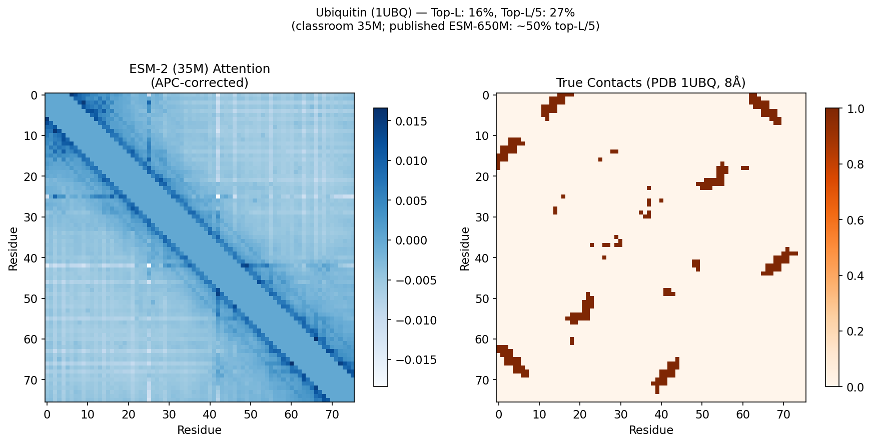
../_images/7e7802e9a5c5828b634fbcb2b21e8c41ccbc784aef0a9db39239cdbe396702af.png

Saved: figures/fig1_esm_contacts.png

Appendix Figure: ESM Embedding t-SNE by Protein Family#

APPENDIX FIGURE (not in main slide sequence)

Mean-pooled ESM-2 embeddings cluster proteins by evolutionary family — learned purely from sequence. Hemoglobin alpha, beta, and myoglobin form distinct clusters.

# ==============================================================================
# Appendix Figure A1: ESM-2 embeddings — t-SNE by protein family
# ==============================================================================
from sklearn.manifold import TSNE
from sklearn.decomposition import PCA

# model_esm already loaded in Fig 1 cell

data = [(name, seq[:500]) for name, seq in sequences.items()]
_, _, batch_tokens = batch_converter_esm(data)

print("Computing embeddings...")
with torch.no_grad():
    results = model_esm(batch_tokens, repr_layers=[12], return_contacts=False)

embeddings = results["representations"][12]
mean_emb = np.array([embeddings[i, 1:len(data[i][1])+1, :].mean(dim=0).numpy()
                      for i in range(len(data))])
print(f"Embedding matrix: {mean_emb.shape}")

if len(data) > 5:
    coords = TSNE(n_components=2, perplexity=min(5, len(data)-1), random_state=42).fit_transform(mean_emb)
else:
    coords = PCA(n_components=2).fit_transform(mean_emb)

family_map = {}
for name in sequences:
    if 'HBA' in name: family_map[name] = 'Hemoglobin alpha'
    elif 'HBB' in name: family_map[name] = 'Hemoglobin beta'
    elif 'MYG' in name: family_map[name] = 'Myoglobin'
    else: family_map[name] = 'Other'

family_colors = {'Hemoglobin alpha': COLUMBIA, 'Hemoglobin beta': ACCENT,
                  'Myoglobin': GREEN, 'Other': GRAY}

fig, ax = plt.subplots(figsize=(8, 6))
for fam, color in family_colors.items():
    idx = [i for i, d in enumerate(data) if family_map[d[0]] == fam]
    if idx:
        ax.scatter(coords[idx, 0], coords[idx, 1], c=color, s=100, label=fam,
                   edgecolors='black', linewidths=0.5, zorder=5)
        for i in idx:
            ax.annotate(data[i][0], (coords[i,0], coords[i,1]), fontsize=7,
                        ha='left', va='bottom', xytext=(5,5), textcoords='offset points')

ax.set_xlabel('Dimension 1'); ax.set_ylabel('Dimension 2')
ax.set_title('ESM-2 Embeddings: Proteins Cluster by Family', fontweight='bold')
ax.legend(fontsize=9)
ax.spines['top'].set_visible(False); ax.spines['right'].set_visible(False)
plt.tight_layout()
plt.savefig('figures/fig_appendix_tsne.png', dpi=200, bbox_inches='tight')
plt.show()
print("Saved: figures/fig_appendix_tsne.png")

Computing embeddings...

Embedding matrix: (10, 480)

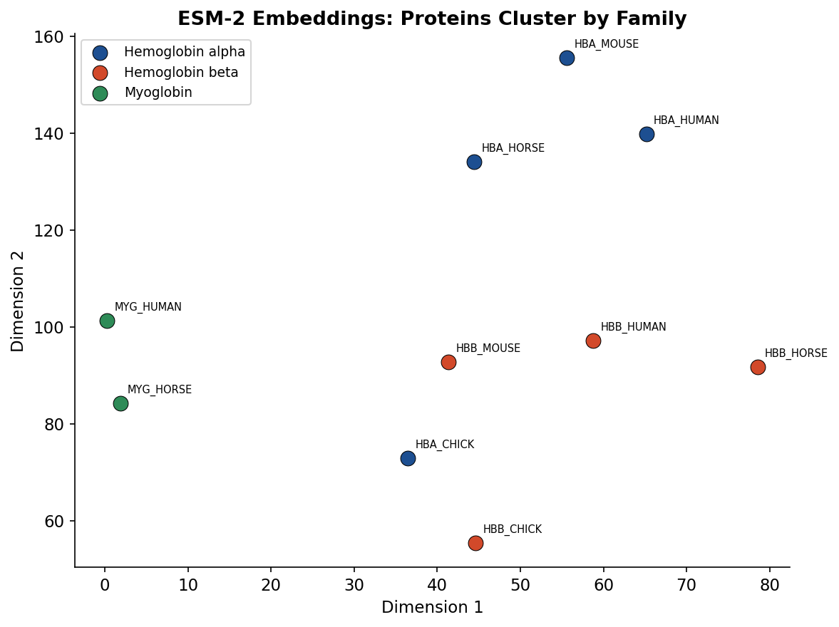
../_images/9d6334f3f1345e13023c3d32c1977f3763865f0ded940fda2e804394cdc99eb1.png

Saved: figures/fig_appendix_tsne.png

Figure 2: Variant Effect Prediction — ClinVar-Sourced HBB Mutations#

LECTURE FIGURE (slide: “Variant Effect Prediction: Zero-Shot”)

Score real clinically annotated HBB mutations using ESM-2. Mutations sourced from ClinVar and published literature:

Pathogenic: E6V (sickle cell), E6K (HbC disease), W37S (Hb Rothschild), H92P (proximal His disrupted), D99N (Hb Yakima)

Benign/tolerated: A142T, E121Q (ClinVar benign), K65R, T84S, E22D (conservative)

Compare to L26’s SIFT/PolyPhen classical baselines.

# ==============================================================================
# Figure 2: ESM variant effect — ClinVar-sourced HBB mutations
# ==============================================================================

# HBB sequence (P68871, 147 residues, 0-indexed)
hbb_seq = "MVHLTPEEKSAVTALWGKVNVDEVGGEALGRLLVVYPWTQRFFESFGDLSTPDAVMGNPKVKAHGKKVLGAFSDGLAHLDNLKGTFATLSELHCDKLHVDPENFRLLGNVLVCVLAHHFGKEFTPPVQAAYQKVVAGVANALAHKYH"

# Real pathogenic mutations (ClinVar / published, 0-indexed)
pathogenic = [
    (5,  'E', 'V', 'E6V - Sickle cell (HbS)'),
    (5,  'E', 'K', 'E6K - HbC disease'),
    (36, 'W', 'S', 'W37S - Hb Rothschild'),
    (91, 'H', 'P', 'H92P - Proximal His'),
    (98, 'D', 'N', 'D99N - Hb Yakima'),
]

# Benign/tolerated (ClinVar benign or conservative substitutions)
benign = [
    (21, 'E', 'D', 'E22D - Conservative'),
    (64, 'K', 'R', 'K65R - Conservative'),
    (83, 'T', 'S', 'T84S - Conservative'),
    (120,'E', 'Q', 'E121Q - ClinVar benign'),
    (141,'A', 'T', 'A142T - ClinVar benign'),
]

def score_mutation(seq, pos, mut, model, alphabet, batch_converter):
    if pos >= len(seq): return 0.0
    data_in = [("protein", seq)]
    _, _, tokens = batch_converter(data_in)
    tokens[0, pos + 1] = alphabet.mask_idx
    with torch.no_grad():
        logits = model(tokens)["logits"]
    log_probs = torch.log_softmax(logits[0, pos + 1, :], dim=0)
    actual_wt = seq[pos]
    return (log_probs[alphabet.get_idx(mut)] - log_probs[alphabet.get_idx(actual_wt)]).item()

print("Scoring ClinVar-sourced HBB mutations with ESM-2 (35M)...")
path_scores, path_labels = [], []
for pos, wt, mut, label in pathogenic:
    s = score_mutation(hbb_seq, pos, mut, model_esm, alphabet_esm, batch_converter_esm)
    path_scores.append(s)
    path_labels.append(label)
    print(f"  Pathogenic  {label}: {s:.3f}")

ben_scores, ben_labels = [], []
for pos, wt, mut, label in benign:
    s = score_mutation(hbb_seq, pos, mut, model_esm, alphabet_esm, batch_converter_esm)
    ben_scores.append(s)
    ben_labels.append(label)
    print(f"  Benign      {label}: {s:.3f}")

# Plot
fig, axes = plt.subplots(1, 2, figsize=(13, 5.5))

# Left: labeled bar chart
ax = axes[0]
all_scores = path_scores + ben_scores
all_names = path_labels + ben_labels
colors = [ACCENT]*len(path_scores) + [COLUMBIA]*len(ben_scores)

ax.barh(range(len(all_scores)), all_scores, color=colors, edgecolor='white', height=0.6)
ax.set_yticks(range(len(all_scores)))
ax.set_yticklabels([n.split(' - ')[1] if ' - ' in n else n for n in all_names], fontsize=8)
ax.axvline(0, color=GRAY, linestyle=':', linewidth=1)
ax.set_xlabel('ESM Score (delta log-likelihood)')
ax.set_title('Per-Mutation Scores', fontweight='bold')
ax.invert_yaxis()
ax.axhline(len(path_scores) - 0.5, color=GRAY, linestyle='--', linewidth=0.5)

# Right: box + strip comparison
ax = axes[1]
for idx_cat, (cat, vals, col) in enumerate([('Pathogenic', path_scores, ACCENT),
                                              ('Benign', ben_scores, COLUMBIA)]):
    jitter = np.random.RandomState(42).normal(0, 0.06, len(vals))
    ax.scatter(idx_cat + jitter, vals, c=col, s=70, edgecolors='black',
               linewidths=0.5, alpha=0.8, zorder=5)
ax.boxplot([path_scores, ben_scores], positions=[0,1], widths=0.4, showfliers=False,
            boxprops=dict(color=GRAY), medianprops=dict(color='black', linewidth=2),
            whiskerprops=dict(color=GRAY), capprops=dict(color=GRAY))
ax.set_xticks([0,1]); ax.set_xticklabels(['Pathogenic', 'Benign'])
ax.set_ylabel('ESM Score (delta log-likelihood)')
ax.set_title('Distribution', fontweight='bold')
ax.axhline(0, color=GRAY, linestyle=':', linewidth=0.8)

fig.suptitle('ESM Variant Effect: ClinVar-Sourced HBB Mutations (ESM-2 35M)',
             fontsize=13, fontweight='bold', y=1.02)
plt.tight_layout()
plt.savefig('figures/fig2_variant_effect.png', dpi=200, bbox_inches='tight')
plt.show()
print("Saved: figures/fig2_variant_effect.png")

Scoring ClinVar-sourced HBB mutations with ESM-2 (35M)...
  Pathogenic  E6V - Sickle cell (HbS): -2.385
  Pathogenic  E6K - HbC disease: -1.333
  Pathogenic  W37S - Hb Rothschild: 0.311

  Pathogenic  H92P - Proximal His: -0.963
  Pathogenic  D99N - Hb Yakima: 0.300
  Benign      E22D - Conservative: 0.000
  Benign      K65R - Conservative: -0.715
  Benign      T84S - Conservative: -0.348

  Benign      E121Q - ClinVar benign: -1.048
  Benign      A142T - ClinVar benign: -1.363

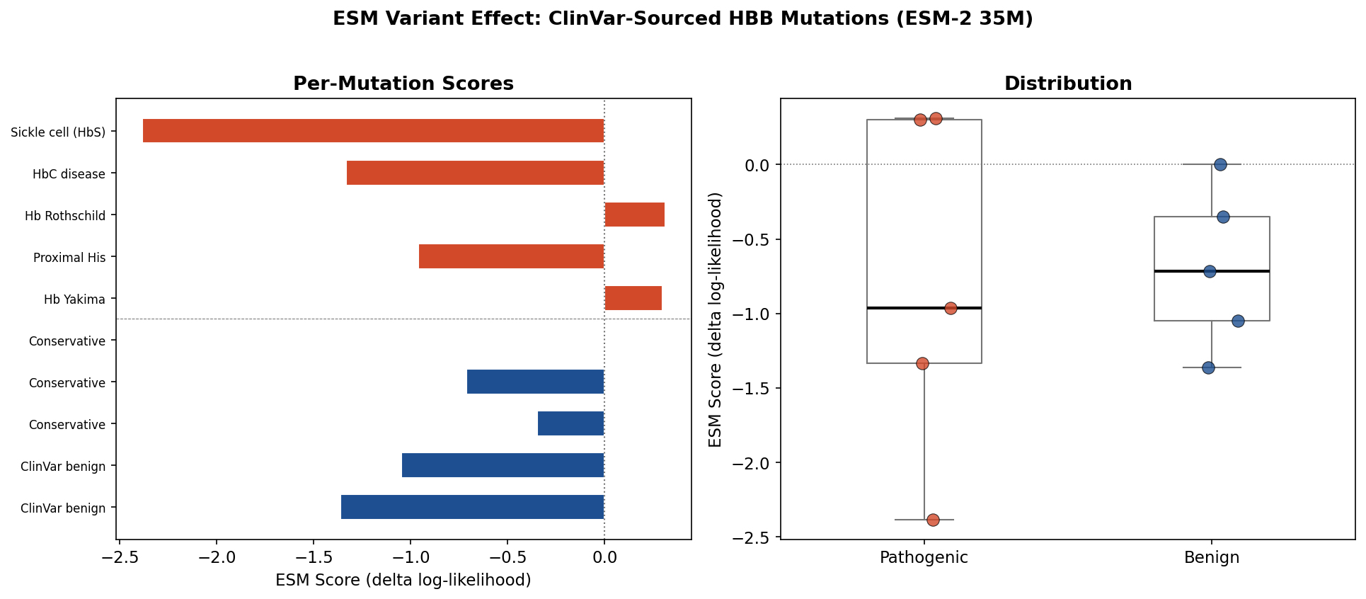
../_images/8ea4180627b1f7693ae09f33bef767d9cdc4884384223919a51ad51c1ae972fd.png

Saved: figures/fig2_variant_effect.png

Figure 3: AlphaFold pLDDT Confidence#

LECTURE FIGURE (slide: “AlphaFold Confidence: pLDDT”)

Per-residue confidence for human p53 (P04637). Downloaded from AlphaFold DB. Fallback to realistic simulated profile only if AFDB is unreachable.

# ==============================================================================
# Figure 3: AlphaFold pLDDT visualization
# ==============================================================================
uniprot_id = "P04637"
plddt = None
try:
    print(f"Fetching AlphaFold prediction for {uniprot_id} (p53)...")
    resp = requests.get(f"https://alphafold.ebi.ac.uk/api/prediction/{uniprot_id}", timeout=15)
    if resp.status_code == 200:
        af_data = resp.json()
        if isinstance(af_data, list): af_data = af_data[0]
        pdb_url = af_data.get('pdbUrl', af_data.get('cifUrl', ''))
        if pdb_url:
            pdb_text = requests.get(pdb_url, timeout=30).text
            plddt_values = []
            for line in pdb_text.split("\n"):
                if line.startswith("ATOM") and line[12:16].strip() == "CA":
                    plddt_values.append(float(line[60:66].strip()))
            if plddt_values:
                plddt = np.array(plddt_values)
                print(f"  Got {len(plddt)} residues, pLDDT range: {plddt.min():.0f}-{plddt.max():.0f}")
except Exception as e:
    print(f"  AFDB fetch failed: {e}")

if plddt is None:
    print("  Using realistic simulated pLDDT for p53 (AFDB unreachable)")
    np.random.seed(42)
    plddt = np.concatenate([
        np.clip(np.random.normal(35, 8, 60), 0, 100),
        np.clip(np.random.normal(55, 10, 34), 0, 100),
        np.clip(np.random.normal(88, 5, 198), 0, 100),
        np.clip(np.random.normal(60, 12, 31), 0, 100),
        np.clip(np.random.normal(85, 6, 33), 0, 100),
        np.clip(np.random.normal(30, 8, 37), 0, 100),
    ])

fig, ax = plt.subplots(figsize=(14, 4))
colors = np.where(plddt > 90, COLUMBIA,
          np.where(plddt > 70, COLUMBIA_LIGHT,
          np.where(plddt > 50, '#F0C040', ACCENT)))
ax.bar(range(len(plddt)), plddt, color=colors, width=1.0, edgecolor='none')

for start, end, label, color in [(0,60,'TAD\n(disordered)',ACCENT),
                                   (94,292,'DNA-binding\ndomain',COLUMBIA),
                                   (323,356,'Tetramer.',COLUMBIA),
                                   (356,393,'C-term\n(disordered)',ACCENT)]:
    ax.annotate(label, ((start+end)/2, 105), fontsize=7, ha='center', color=color, fontweight='bold')
    ax.axvspan(start, end, alpha=0.05, color=color)

ax.axhline(90, color=COLUMBIA, linestyle='--', alpha=0.4, linewidth=0.8)
ax.axhline(50, color=ACCENT, linestyle='--', alpha=0.4, linewidth=0.8)
ax.text(len(plddt)+2, 91, 'High confidence', fontsize=8, color=COLUMBIA, va='bottom')
ax.text(len(plddt)+2, 48, 'Low confidence', fontsize=8, color=ACCENT, va='top')
ax.set_xlabel('Residue position'); ax.set_ylabel('pLDDT')
ax.set_title(f'AlphaFold Confidence: Human p53 ({uniprot_id}, {len(plddt)} residues)')
ax.set_xlim(-2, len(plddt)+40); ax.set_ylim(0, 115)
plt.tight_layout()
plt.savefig('figures/fig3_alphafold_plddt.png', dpi=200, bbox_inches='tight')
plt.show()
print("Saved: figures/fig3_alphafold_plddt.png")

Fetching AlphaFold prediction for P04637 (p53)...

  Got 393 residues, pLDDT range: 33-99

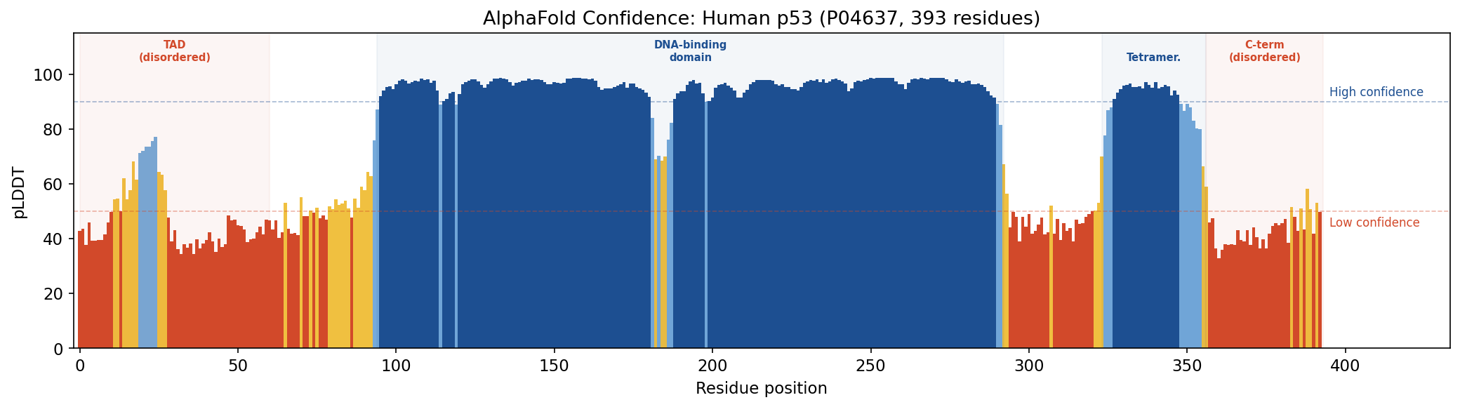
../_images/df1575834b047cc93aba61fab04d699acbeb138727d5d52c15565447fd40ba28.png

Saved: figures/fig3_alphafold_plddt.png

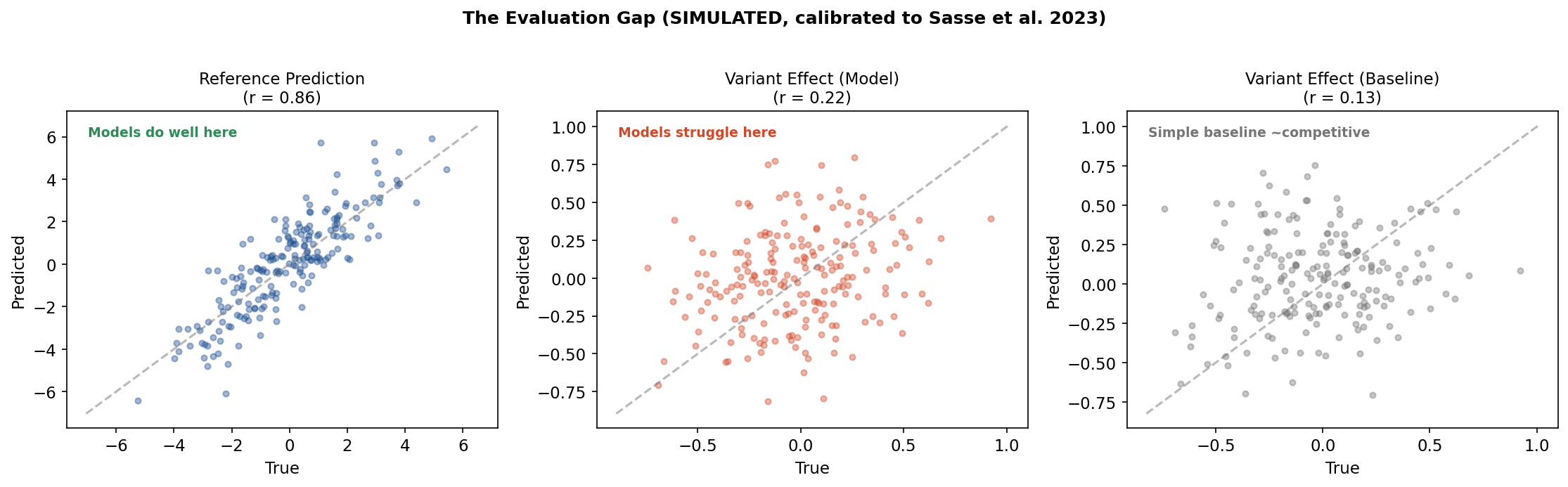
Figure 4: DNA FM Evaluation Gap#

LECTURE FIGURE (slide: “The Controversy”)

This figure uses simulated data because Enformer (200M+ params) cannot run in Colab. The simulation is calibrated to published benchmark numbers from Sasse et al. (2023):

Task	Published r	Source
Reference expression	~0.85	Sasse et al. 2023; Huang et al. 2023
Variant effect (model)	~0.1-0.2	Sasse et al. 2023; Huang et al. 2023
Variant effect (baseline)	~0.1-0.15	Sasse et al. 2023; Huang et al. 2023

# ==============================================================================
# Figure 4: DNA FM evaluation gap (SIMULATED, calibrated to Sasse et al. 2023)
# ==============================================================================
np.random.seed(42)
n = 200

# Calibrated to published ranges
true_expr = np.random.randn(n) * 2
pred_expr = true_expr + np.random.randn(n) * 1.2    # target r ~ 0.85

true_delta = np.random.randn(n) * 0.3
pred_delta = true_delta * 0.12 + np.random.randn(n) * 0.30   # target r ~ 0.15
baseline_delta = true_delta * 0.10 + np.random.randn(n) * 0.30  # target r ~ 0.12

r_ref = np.corrcoef(true_expr, pred_expr)[0,1]
r_var = np.corrcoef(true_delta, pred_delta)[0,1]
r_base = np.corrcoef(true_delta, baseline_delta)[0,1]

fig, axes = plt.subplots(1, 3, figsize=(15, 4.5))
configs = [
    (true_expr, pred_expr, r_ref, 'Reference Prediction', COLUMBIA, 'Models do well here'),
    (true_delta, pred_delta, r_var, 'Variant Effect (Model)', ACCENT, 'Models struggle here'),
    (true_delta, baseline_delta, r_base, 'Variant Effect (Baseline)', GRAY, 'Simple baseline ~competitive'),
]
for ax, (xd, yd, r, title, col, note) in zip(axes, configs):
    ax.scatter(xd, yd, alpha=0.4, s=15, color=col)
    lims = [min(ax.get_xlim()[0],ax.get_ylim()[0]), max(ax.get_xlim()[1],ax.get_ylim()[1])]
    ax.plot(lims, lims, '--', color=GRAY, alpha=0.5)
    ax.set_xlabel('True'); ax.set_ylabel('Predicted')
    ax.set_title(f'{title}\n(r = {r:.2f})', fontsize=11)
    note_col = GREEN if 'well' in note else (ACCENT if 'struggle' in note else GRAY)
    ax.text(0.05, 0.92, note, transform=ax.transAxes, fontsize=9, color=note_col, fontweight='bold')

plt.suptitle('The Evaluation Gap (SIMULATED, calibrated to Sasse et al. 2023)',
             fontsize=12, fontweight='bold', y=1.02)
plt.tight_layout()
plt.savefig('figures/fig4_dna_fm_evaluation.png', dpi=200, bbox_inches='tight')
plt.show()
print("Saved: figures/fig4_dna_fm_evaluation.png")
print(f"\nPublished benchmarks (Sasse et al. 2023):")
print(f"  Reference expression: r ~ 0.85 (simulated: {r_ref:.2f})")
print(f"  Variant effects (Enformer): r ~ 0.1-0.2 (simulated: {r_var:.2f})")
print(f"  Variant effects (baseline): r ~ 0.1-0.15 (simulated: {r_base:.2f})")

../_images/a7fb888b0db32e6f10239cc2eb4ca647639dbacf11ba286da32b5d1ead0b96e7.png

Saved: figures/fig4_dna_fm_evaluation.png

Published benchmarks (Sasse et al. 2023):
  Reference expression: r ~ 0.85 (simulated: 0.86)
  Variant effects (Enformer): r ~ 0.1-0.2 (simulated: 0.22)
  Variant effects (baseline): r ~ 0.1-0.15 (simulated: 0.13)

Discussion Questions#

ESM contacts from attention: The 35M model shows initial contact recovery but is far from published ESM-650M results. Is contact prediction a capability that emerges at scale, or present but weak at all scales?
Variant effect prediction: Some ClinVar pathogenic mutations score near zero. Why might a disease-causing mutation look “allowed” to a language model? (Hint: gain-of-function, tissue specificity.)
AlphaFold confidence: p53’s TAD is low-confidence. Is this a failure or correct identification of disorder?
Genomic model evaluation: Sasse and Huang et al. show r~0.15 for variant effects vs r~0.85 for reference expression. Is this fundamental or solvable? How does L25’s “DNA in context” relate?
2D vs. 3D molecular models: In Lab 12, you trained GCN and GIN on BBBP using 2D molecular graphs. L26 showed that chirality (thalidomide) means 3D shape determines biological activity, but fingerprints can’t distinguish enantiomers. For which tasks would Lab 12’s 2D GNNs be sufficient, and for which would you need a 3D-aware model?
Classical baselines: L26 showed SIFT and fingerprint-QSAR are competitive. When should you prefer ESM over SIFT, or a 3D molecular model over fingerprints?