🔬 Lab 8: Time-to-Event Prediction (Survival Analysis)

BINF 4002 – Machine Learning for Health

Labs 6–7 changed the target type (multi-class labels, continuous values) but kept the fundamental assumption that we observe the true outcome for every patient. In clinical reality, this is often false. Patients drop out of studies, are lost to follow-up, or the study ends before the event occurs. These patients’ outcomes are censored — we know their event time is at least as long as their observation time, but we don’t know the actual event time.

Standard regression and classification both fail here. Regression on observed times is biased (censored patients look like short survivors). Binary classification (event yes/no by some cutoff) throws away temporal information. Survival analysis is the proper framework: it models the time until an event while correctly accounting for censoring.

This lab introduces a genuinely new loss function — the Cox partial likelihood — that cannot be reduced to any loss from Labs 1–7.

Learning Objectives

1. Understand right-censoring and why standard regression/classification fails

2. Implement the Kaplan-Meier estimator and Cox partial likelihood loss by hand

3. Fit and evaluate Cox PH and Random Survival Forest models

4. Evaluate with concordance index (C-index) and calibration via Kaplan-Meier curves

Set-up

Install dependencies

This lab uses scikit-survival, a library for survival analysis built on top of scikit-learn. It provides datasets, models, and evaluation metrics for censored time-to-event data.

# Install scikit-survival (may take 1-2 minutes on Colab)
# (pip install handled by the book's isolated env)

Imports and Helper Functions

import numpy as np
import pandas as pd
import matplotlib.pyplot as plt
import matplotlib.gridspec as gridspec
import seaborn as sns
import warnings
warnings.filterwarnings('ignore')

plt.rcParams['figure.dpi'] = 110
plt.rcParams['axes.spines.top'] = False
plt.rcParams['axes.spines.right'] = False
sns.set_palette("Set2")

from sksurv.datasets import load_gbsg2
from sksurv.preprocessing import OneHotEncoder

print("✅ All imports successful!")

✅ All imports successful!

Load and prepare the GBSG2 dataset

The German Breast Cancer Study Group 2 (GBSG2) dataset contains 686 breast cancer patients with 8 clinical features and a time-to-event outcome: time to cancer recurrence (in days), with ~44% of patients experiencing recurrence (events) and ~56% censored (event-free at last follow-up).

This keeps the breast cancer theme from Labs 0–7 while introducing real censoring.

# ── Load GBSG2 dataset ───────────────────────────────────────────────────────
X_raw, y = load_gbsg2()

# y is a structured array with fields: 'cens' (event indicator) and 'time'
event = y['cens']     # True = recurrence observed, False = censored
time  = y['time']     # days until recurrence or last follow-up

print(f"Dataset: {X_raw.shape[0]} patients, {X_raw.shape[1]} features")
print(f"Events: {event.sum()} ({event.mean():.1%}) experienced recurrence")
print(f"Censored: {(~event).sum()} ({(~event).mean():.1%}) event-free at last follow-up")
print(f"\nFollow-up time: {time.min():.0f} – {time.max():.0f} days "
      f"({time.min()/365.25:.1f} – {time.max()/365.25:.1f} years)")
print(f"\nFeatures:")
print(X_raw.dtypes.to_string())

Dataset: 686 patients, 8 features
Events: 299 (43.6%) experienced recurrence
Censored: 387 (56.4%) event-free at last follow-up

Follow-up time: 8 – 2659 days (0.0 – 7.3 years)

Features:
age          float64
estrec       float64
horTh       category
menostat    category
pnodes       float64
progrec      float64
tgrade      category
tsize        float64

# ── Preprocess: one-hot encode categorical features ──────────────────────────
encoder = OneHotEncoder()
X_encoded = encoder.fit_transform(X_raw)

feature_names = list(X_encoded.columns)
print(f"After encoding: {X_encoded.shape[1]} features")
print(f"Columns: {feature_names}")

# ── Train/val/test split ──────────────────────────────────────────────────────
from sklearn.model_selection import train_test_split

# First split: 70% train, 30% temp
X_train, X_temp, y_train, y_temp = train_test_split(
    X_encoded.values, y, test_size=0.30, random_state=42)

# Second split: 15% val, 15% test
X_val, X_test, y_val, y_test = train_test_split(
    X_temp, y_temp, test_size=0.50, random_state=42)

print(f"\nTrain: {len(y_train)} ({y_train['cens'].mean():.1%} events)")
print(f"Val:   {len(y_val)} ({y_val['cens'].mean():.1%} events)")
print(f"Test:  {len(y_test)} ({y_test['cens'].mean():.1%} events)")

After encoding: 9 features
Columns: ['age', 'estrec', 'horTh=yes', 'menostat=Post', 'pnodes', 'progrec', 'tgrade=II', 'tgrade=III', 'tsize']

Train: 480 (44.8% events)
Val:   103 (44.7% events)
Test:  103 (36.9% events)

---

Background — What Is Survival Analysis?

Before diving into specific estimators and models, let’s build intuition for what survival analysis is and why it matters.

The central question: Given a group of patients, what is the probability that a patient survives (remains event-free) beyond time \(t\)? This is captured by the survival function \(S(t) = P(T > t)\), where \(T\) is the (possibly unobserved) time until the event of interest (death, recurrence, readmission, etc.).

Related quantities:

• The hazard function \(h(t)\) describes the instantaneous risk of the event at time \(t\), given survival up to \(t\). Think of it as the “danger level” at each moment.

• The cumulative hazard \(H(t) = \int_0^t h(s) \, ds\) accumulates risk over time.

• These are all related: \(S(t) = \exp(-H(t))\), so higher cumulative hazard means lower survival.

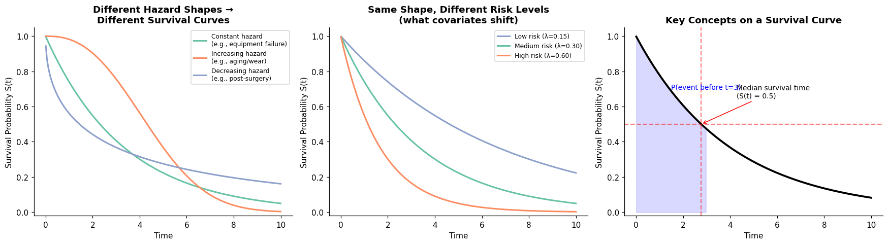
Typical shapes of survival curves:

• A constant hazard (e.g., a lightbulb burning out) produces an exponential survival curve: \(S(t) = e^{-\lambda t}\). The curve drops steadily.

• An increasing hazard (e.g., aging-related disease) produces a curve that drops slowly at first, then faster — the longer you survive, the higher your instantaneous risk.

• A decreasing hazard (e.g., post-surgery mortality) drops steeply early on, then flattens. The most dangerous period is right after the event (surgery), and risk decreases over time.

• A bathtub hazard (e.g., overall human mortality) is high in infancy, low in middle age, and high again in old age.

Understanding these shapes is essential: the shape of the survival curve tells a clinical story. Let’s visualize some examples before working with real data.

# ── Example survival curves — building intuition ─────────────────────────────
fig, axes = plt.subplots(1, 3, figsize=(16, 4.5))

t = np.linspace(0.01, 10, 200)

# (a) Different hazard shapes → different survival curves
ax = axes[0]
# Constant hazard (exponential): h(t) = 0.3
S_const = np.exp(-0.3 * t)
# Increasing hazard (Weibull, shape > 1): h(t) ∝ t^1.5
S_incr = np.exp(-(t / 5) ** 2.5)
# Decreasing hazard (Weibull, shape < 1): h(t) ∝ t^{-0.5}
S_decr = np.exp(-(t / 3) ** 0.5)

ax.plot(t, S_const, linewidth=2, label='Constant hazard\n(e.g., equipment failure)')
ax.plot(t, S_incr, linewidth=2, label='Increasing hazard\n(e.g., aging/wear)')
ax.plot(t, S_decr, linewidth=2, label='Decreasing hazard\n(e.g., post-surgery)')
ax.set_xlabel('Time')
ax.set_ylabel('Survival Probability S(t)')
ax.set_title('Different Hazard Shapes →\nDifferent Survival Curves', fontweight='bold')
ax.legend(fontsize=8)
ax.set_ylim(-0.02, 1.05)

# (b) Same shape, different risk levels (covariate effect)
ax = axes[1]
ax.plot(t, np.exp(-0.15 * t), linewidth=2, label='Low risk (λ=0.15)', color=sns.color_palette('Set2')[2])
ax.plot(t, np.exp(-0.30 * t), linewidth=2, label='Medium risk (λ=0.30)', color=sns.color_palette('Set2')[0])
ax.plot(t, np.exp(-0.60 * t), linewidth=2, label='High risk (λ=0.60)', color=sns.color_palette('Set2')[1])
ax.set_xlabel('Time')
ax.set_ylabel('Survival Probability S(t)')
ax.set_title('Same Shape, Different Risk Levels\n(what covariates shift)', fontweight='bold')
ax.legend(fontsize=8)
ax.set_ylim(-0.02, 1.05)

# (c) Annotated survival curve with key concepts
ax = axes[2]
S_demo = np.exp(-0.25 * t)
ax.plot(t, S_demo, linewidth=2.5, color='black')
ax.axhline(0.5, color='red', linestyle='--', alpha=0.5)
median_t = np.log(2) / 0.25
ax.axvline(median_t, color='red', linestyle='--', alpha=0.5)
ax.annotate('Median survival time\n(S(t) = 0.5)', xy=(median_t, 0.5),
            xytext=(median_t + 1.5, 0.65), fontsize=9,
            arrowprops=dict(arrowstyle='->', color='red'))
ax.fill_between(t[t <= 3], S_demo[t <= 3], alpha=0.15, color='blue')
ax.annotate('P(event before t=3)', xy=(1.5, 0.7), fontsize=9, color='blue')
ax.set_xlabel('Time')
ax.set_ylabel('Survival Probability S(t)')
ax.set_title('Key Concepts on a Survival Curve', fontweight='bold')
ax.set_ylim(-0.02, 1.05)

plt.tight_layout()
plt.show()

print("Key takeaways:")
print("  • The survival curve S(t) starts at 1 and decreases toward 0")
print("  • The SHAPE tells you about the hazard pattern (constant, increasing, decreasing)")
print("  • The LEVEL tells you about the overall risk (higher risk → curve drops faster)")
print("  • Median survival = time when S(t) crosses 0.5 (half the population has had the event)")
print("  • Clinical decisions often hinge on S(t) at specific time points (e.g., 5-year survival rate)")

Key takeaways:
  • The survival curve S(t) starts at 1 and decreases toward 0
  • The SHAPE tells you about the hazard pattern (constant, increasing, decreasing)
  • The LEVEL tells you about the overall risk (higher risk → curve drops faster)
  • Median survival = time when S(t) crosses 0.5 (half the population has had the event)
  • Clinical decisions often hinge on S(t) at specific time points (e.g., 5-year survival rate)

---

Part 1 — Why Censoring Breaks Standard Approaches

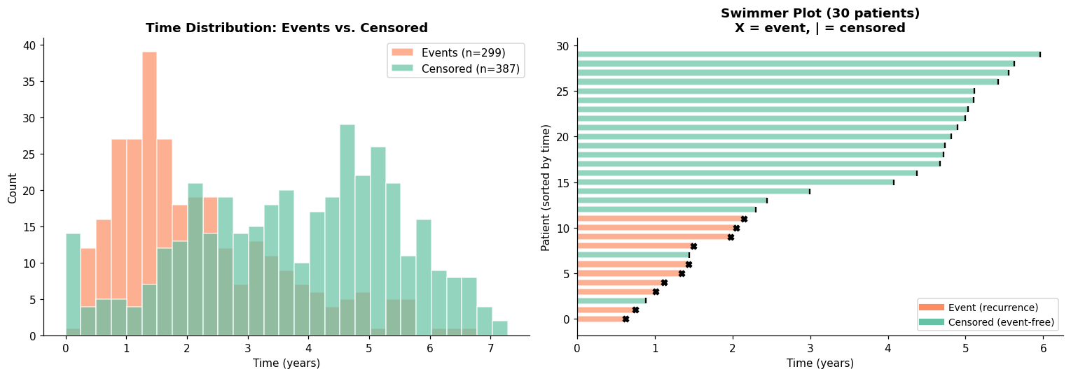
Before introducing survival models, we need to understand why we can’t just use standard regression or classification on time-to-event data. The answer is censoring: for many patients, we don’t observe the actual event time — we only know that it’s at least as long as their follow-up time.

# ── Visualize event-time distribution ─────────────────────────────────────────
fig, axes = plt.subplots(1, 2, figsize=(14, 5))

# Histogram: events vs. censored
time_yrs = time / 365.25
event_times = time_yrs[event]
censor_times = time_yrs[~event]

bins = np.linspace(0, time_yrs.max(), 30)
axes[0].hist(event_times, bins=bins, alpha=0.7, label=f'Events (n={event.sum()})',
             color=sns.color_palette('Set2')[1], edgecolor='white')
axes[0].hist(censor_times, bins=bins, alpha=0.7, label=f'Censored (n={(~event).sum()})',
             color=sns.color_palette('Set2')[0], edgecolor='white')
axes[0].set_xlabel('Time (years)')
axes[0].set_ylabel('Count')
axes[0].set_title('Time Distribution: Events vs. Censored', fontweight='bold')
axes[0].legend()

# Swimmer plot: 30 random patients
np.random.seed(42)
swim_idx = np.random.choice(len(time), 30, replace=False)
swim_idx = swim_idx[np.argsort(time[swim_idx])]

for i, idx in enumerate(swim_idx):
    color = sns.color_palette('Set2')[1] if event[idx] else sns.color_palette('Set2')[0]
    marker = 'X' if event[idx] else '|'
    axes[1].barh(i, time[idx] / 365.25, height=0.7, color=color, alpha=0.7, edgecolor='white')
    axes[1].scatter(time[idx] / 365.25, i, marker=marker, color='black', s=30, zorder=3)

axes[1].set_xlabel('Time (years)')
axes[1].set_ylabel('Patient (sorted by time)')
axes[1].set_title('Swimmer Plot (30 patients)\nX = event, | = censored', fontweight='bold')

# Custom legend
from matplotlib.lines import Line2D
legend_elements = [
    Line2D([0], [0], color=sns.color_palette('Set2')[1], lw=6, label='Event (recurrence)'),
    Line2D([0], [0], color=sns.color_palette('Set2')[0], lw=6, label='Censored (event-free)'),
]
axes[1].legend(handles=legend_elements, fontsize=9, loc='lower right')

plt.tight_layout()
plt.show()

print("Censored patients (|): we know they survived AT LEAST this long.")
print("Their true event time could be any time AFTER the censoring time.")

Censored patients (|): we know they survived AT LEAST this long.
Their true event time could be any time AFTER the censoring time.

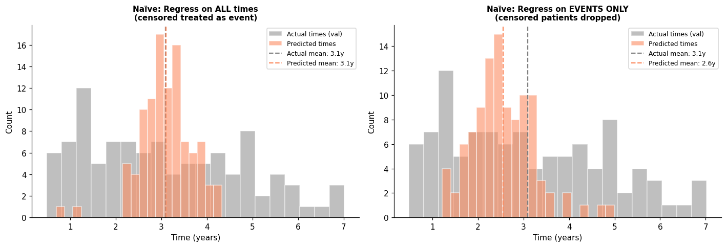
# ── Demonstrate the naïve failure ────────────────────────────────────────────
# Approach 1: Regression — just predict time, ignoring censoring
# Approach 2: Drop censored patients and regress on events only
# Both are biased!

from sklearn.linear_model import LinearRegression
from sklearn.metrics import mean_absolute_error

# Naïve 1: Treat all times as true event times
lr_naive_all = LinearRegression()
lr_naive_all.fit(X_train, y_train['time'])
pred_naive_all = lr_naive_all.predict(X_val)

# Naïve 2: Drop censored, train only on events
event_mask_train = y_train['cens']
lr_naive_events = LinearRegression()
lr_naive_events.fit(X_train[event_mask_train], y_train[event_mask_train]['time'])
pred_naive_events = lr_naive_events.predict(X_val)

# Show the bias
fig, axes = plt.subplots(1, 2, figsize=(13, 4.5))

# Compare predicted distributions
val_event_times = y_val[y_val['cens']]['time']

for ax, preds, title in zip(axes,
    [pred_naive_all, pred_naive_events],
    ['Naïve: Regress on ALL times\n(censored treated as event)',
     'Naïve: Regress on EVENTS ONLY\n(censored patients dropped)']):

    ax.hist(y_val['time'] / 365.25, bins=20, alpha=0.5, label='Actual times (val)',
            color='gray', edgecolor='white')
    ax.hist(preds / 365.25, bins=20, alpha=0.6, label='Predicted times',
            color=sns.color_palette('Set2')[1], edgecolor='white')
    ax.axvline(y_val['time'].mean() / 365.25, color='gray', linestyle='--',
               label=f'Actual mean: {y_val["time"].mean()/365.25:.1f}y')
    ax.axvline(preds.mean() / 365.25, color=sns.color_palette('Set2')[1], linestyle='--',
               label=f'Predicted mean: {preds.mean()/365.25:.1f}y')
    ax.set_xlabel('Time (years)')
    ax.set_ylabel('Count')
    ax.set_title(title, fontweight='bold', fontsize=10)
    ax.legend(fontsize=8)

plt.tight_layout()
plt.show()

print("⚠️ Both naïve approaches are biased:")
print("  • Treating censored times as true events: systematically underestimates survival")
print("    (a patient censored at 3 years might have survived 10 years)")
print("  • Dropping censored patients: discards >50% of data, biases toward shorter times")
print("    (events tend to happen earlier; survivors are disproportionately censored)")

⚠️ Both naïve approaches are biased:
  • Treating censored times as true events: systematically underestimates survival
    (a patient censored at 3 years might have survived 10 years)
  • Dropping censored patients: discards >50% of data, biases toward shorter times
    (events tend to happen earlier; survivors are disproportionately censored)

🤔 Reflection 1.1 — The Censoring Problem

1. A patient enrolled in a 5-year study was event-free at 3 years when they moved cities and were lost to follow-up. Their true survival time is at least 3 years. Why is it wrong to label them as “survived 3 years” (regression target) or “no event” (binary classification)?

2. Look at the swimmer plot. Among the patients with the longest bars, are they disproportionately censored or event patients? Why?

3. A colleague suggests: “Just use binary classification — did the patient recur within 5 years, yes or no?” What information does this approach discard? (Hint: consider two patients who both recurred, one at 6 months and one at 4.5 years.)

---

Part 2 — The Kaplan-Meier Estimator

The Kaplan-Meier (KM) estimator is the simplest and most important tool in survival analysis. It estimates the survival function \(S(t) = P(T > t)\) — the probability of surviving beyond time \(t\) — without assuming any parametric form.

At each event time \(t_j\): $\(\hat{S}(t_j) = \hat{S}(t_{j-1}) \cdot \left(1 - \frac{d_j}{n_j}\right)\)$

where:

• \(d_j\) = number of events (recurrences) at time \(t_j\)

• \(n_j\) = number of patients at risk just before \(t_j\) (still alive and uncensored)

• \(\hat{S}(0) = 1\) (everyone starts alive)

The curve drops at each event and stays flat between events. Censored observations reduce the risk set \(n_j\) without causing a drop.

def kaplan_meier_solution(event_indicator, time_to_event):
    """
    Compute the Kaplan-Meier survival function.
    """
    order = np.argsort(time_to_event)
    sorted_time  = time_to_event[order]
    sorted_event = event_indicator[order]

    unique_event_times = np.unique(sorted_time[sorted_event])

    survival_prob = []
    s = 1.0

    for t_j in unique_event_times:
        # n_j = number at risk just before t_j
        n_j = np.sum(sorted_time >= t_j)

        # d_j = number of events at exactly t_j
        d_j = np.sum((sorted_time == t_j) & sorted_event)

        # Update survival probability
        s = s * (1 - d_j / n_j)

        survival_prob.append(s)

    return unique_event_times, np.array(survival_prob)

# Verify
km_t_sol, km_s_sol = kaplan_meier_solution(y_train['cens'], y_train['time'])
km_t_sk, km_s_sk = kaplan_meier_estimator(y_train['cens'], y_train['time'])
common = np.intersect1d(km_t_sol, km_t_sk)
ours_c = km_s_sol[np.isin(km_t_sol, common)]
sk_c = km_s_sk[np.isin(km_t_sk, common)]
print(f"Max diff: {np.max(np.abs(ours_c - sk_c)):.2e}  ✅")

---------------------------------------------------------------------------
NameError                                 Traceback (most recent call last)
Cell In[8], line 30
     26     return unique_event_times, np.array(survival_prob)
     27 
     28 # Verify
     29 km_t_sol, km_s_sol = kaplan_meier_solution(y_train['cens'], y_train['time'])
---> 30 km_t_sk, km_s_sk = kaplan_meier_estimator(y_train['cens'], y_train['time'])
     31 common = np.intersect1d(km_t_sol, km_t_sk)
     32 ours_c = km_s_sol[np.isin(km_t_sol, common)]
     33 sk_c = km_s_sk[np.isin(km_t_sk, common)]

NameError: name 'kaplan_meier_estimator' is not defined

# ── Plot KM curves ───────────────────────────────────────────────────────────
fig, axes = plt.subplots(1, 2, figsize=(14, 5))

# Overall KM curve
ax = axes[0]
ax.step(km_times_ours / 365.25, km_surv_ours, where='post', linewidth=2,
        label='Our implementation', color=sns.color_palette('Set2')[0])
ax.step(km_times_sk / 365.25, km_surv_sk, where='post', linewidth=2,
        linestyle='--', label='sksurv', color=sns.color_palette('Set2')[1])
ax.set_xlabel('Time (years)')
ax.set_ylabel('Survival Probability S(t)')
ax.set_title('Kaplan-Meier Curve (Training Set)', fontweight='bold')
ax.set_ylim(-0.02, 1.05)
ax.legend()

# Stratified by hormonal therapy
ax = axes[1]
# Get horTh feature from raw data for train indices
horTh_train = X_raw.iloc[: , X_raw.columns.get_loc('horTh')]

# Reconstruct which indices went to train
# Simpler: stratify directly on the encoded feature
horTh_col = feature_names.index('horTh=yes')
for val, label, color in [(1, 'Hormonal Therapy', sns.color_palette('Set2')[2]),
                           (0, 'No Hormonal Therapy', sns.color_palette('Set2')[3])]:
    mask = X_train[:, horTh_col] == val
    if mask.sum() > 0:
        t_km, s_km = kaplan_meier_estimator(y_train[mask]['cens'], y_train[mask]['time'])
        ax.step(t_km / 365.25, s_km, where='post', linewidth=2, label=label, color=color)

ax.set_xlabel('Time (years)')
ax.set_ylabel('Survival Probability S(t)')
ax.set_title('KM Curves Stratified by Hormonal Therapy', fontweight='bold')
ax.set_ylim(-0.02, 1.05)
ax.legend()

plt.tight_layout()
plt.show()

# Median survival
median_idx = np.searchsorted(-km_surv_ours, -0.5)
if median_idx < len(km_times_ours):
    print(f"Estimated median recurrence-free survival: {km_times_ours[median_idx]/365.25:.1f} years")
else:
    print("Median survival not reached (>50% of patients are event-free at max follow-up)")

---------------------------------------------------------------------------
NameError                                 Traceback (most recent call last)
Cell In[9], line 6
      2 fig, axes = plt.subplots(1, 2, figsize=(14, 5))
      3 
      4 # Overall KM curve
      5 ax = axes[0]
----> 6 ax.step(km_times_ours / 365.25, km_surv_ours, where='post', linewidth=2,
      7         label='Our implementation', color=sns.color_palette('Set2')[0])
      8 ax.step(km_times_sk / 365.25, km_surv_sk, where='post', linewidth=2,
      9         linestyle='--', label='sksurv', color=sns.color_palette('Set2')[1])

NameError: name 'km_times_ours' is not defined

🤔 Reflection 2.1 — The Kaplan-Meier Estimator

1. The KM estimator makes no assumptions about the shape of the survival curve (it’s completely non-parametric). Why is this useful? When might you want a parametric model instead? (Hint: small sample sizes.)

2. When patients are censored, the “number at risk” \(n_j\) decreases. This means late event-time estimates are based on fewer patients. How does this affect the confidence in the right tail of the KM curve?

3. Look at the stratified KM curves. Does hormonal therapy appear to improve recurrence-free survival? The KM curve doesn’t adjust for confounders — why might the apparent treatment effect be misleading?

---

Part 3 — Cox Proportional Hazards: The Loss Function

The Cox Proportional Hazards (Cox PH) model is the workhorse of survival analysis. It models the hazard function — the instantaneous risk of the event at time \(t\), given that the patient has survived until \(t\):

\[h(t | \mathbf{x}) = h_0(t) \cdot \exp(\boldsymbol{\beta}^\top \mathbf{x})\]

where:

• \(h_0(t)\) is the baseline hazard — left completely unspecified (non-parametric)

• \(\exp(\boldsymbol{\beta}^\top \mathbf{x})\) is the relative risk based on features

• \(\boldsymbol{\beta}\) are the parameters we learn

Key insight: Because \(h_0(t)\) is unspecified, we can’t write a standard likelihood. Cox’s breakthrough was the partial likelihood, which only depends on the ranking of patients within each risk set, not the absolute times:

\[\mathcal{L}_\text{partial} = \prod_{i: \delta_i = 1} \frac{\exp(\boldsymbol{\beta}^\top \mathbf{x}_i)}{\sum_{j \in \mathcal{R}(t_i)} \exp(\boldsymbol{\beta}^\top \mathbf{x}_j)}\]

where \(\delta_i = 1\) means patient \(i\) had an event, and \(\mathcal{R}(t_i)\) is the risk set at time \(t_i\) — all patients still alive and uncensored just before \(t_i\).

def cox_neg_log_partial_likelihood_solution(beta, X, event, time):
    """
    Compute the negative log-partial-likelihood of the Cox model.
    """
    risk_scores = X @ beta
    nll = 0.0

    for i in range(len(time)):
        if not event[i]:
            continue

        risk_set = time >= time[i]

        rs_risk = risk_scores[risk_set]
        max_rs = rs_risk.max()
        log_sum_exp = max_rs + np.log(np.sum(np.exp(rs_risk - max_rs)))

        nll -= risk_scores[i] - log_sum_exp

    return nll

# Verify
nll_sol = cox_neg_log_partial_likelihood_solution(beta_sk, X_train, y_train['cens'], y_train['time'])
nll_null_sol = cox_neg_log_partial_likelihood_solution(np.zeros(X_train.shape[1]), X_train, y_train['cens'], y_train['time'])
print(f"NLL at fitted β: {nll_sol:.2f}")
print(f"NLL at β=0:      {nll_null_sol:.2f}")
print(f"Improvement:     {nll_null_sol - nll_sol:.2f}")

---------------------------------------------------------------------------
NameError                                 Traceback (most recent call last)
Cell In[10], line 23
     19 
     20     return nll
     21 
     22 # Verify
---> 23 nll_sol = cox_neg_log_partial_likelihood_solution(beta_sk, X_train, y_train['cens'], y_train['time'])
     24 nll_null_sol = cox_neg_log_partial_likelihood_solution(np.zeros(X_train.shape[1]), X_train, y_train['cens'], y_train['time'])
     25 print(f"NLL at fitted β: {nll_sol:.2f}")
     26 print(f"NLL at β=0:      {nll_null_sol:.2f}")

NameError: name 'beta_sk' is not defined

# ── Examine Cox model coefficients ───────────────────────────────────────────
coef_df = pd.DataFrame({
    'Feature': feature_names,
    'Coefficient (β)': beta_sk,
    'Hazard Ratio (exp(β))': np.exp(beta_sk)
}).sort_values('Coefficient (β)', ascending=False)

print("Cox PH Model Coefficients:")
print("─" * 60)
print(coef_df.to_string(index=False, float_format='%.4f'))
print("\nInterpretation:")
print("  β > 0 (HR > 1): higher feature value → higher hazard (worse prognosis)")
print("  β < 0 (HR < 1): higher feature value → lower hazard (better prognosis)")
print("  HR = 1.5 means 50% higher instantaneous risk of recurrence")

---------------------------------------------------------------------------
NameError                                 Traceback (most recent call last)
Cell In[11], line 4
      1 # ── Examine Cox model coefficients ───────────────────────────────────────────
      2 coef_df = pd.DataFrame({
      3     'Feature': feature_names,
----> 4     'Coefficient (β)': beta_sk,
      5     'Hazard Ratio (exp(β))': np.exp(beta_sk)
      6 }).sort_values('Coefficient (β)', ascending=False)
      7 

NameError: name 'beta_sk' is not defined

🤔 Reflection 3.1 — The Cox Partial Likelihood

1. The Cox partial likelihood only uses the ranking of patients within each risk set, not the absolute event times. This is what makes it semi-parametric: the baseline hazard \(h_0(t)\) is never estimated. Why is this a strength? When might it be a limitation? (Hint: can the Cox model predict the probability of surviving beyond 5 years without estimating \(h_0\)?)

2. The proportional hazards assumption means that the hazard ratio between any two patients is constant over time. In clinical terms: if patient A has 2× the risk of patient B at year 1, they also have 2× the risk at year 5. When might this be violated? (Hint: think of a treatment whose effect wears off over time.)

3. Look at the hazard ratios. Which features are the strongest prognostic factors? Do the directions make clinical sense?

Random Survival Forests (RSF) — A Brief Overview

Alongside the Cox PH model, we will also use a Random Survival Forest (RSF). This is the survival analysis extension of the random forests you may have seen in classification and regression.

Key ideas:

• Like a standard random forest, RSF builds an ensemble of decision trees, each trained on a bootstrap sample of the data with random feature subsets at each split.

• The splitting criterion is different: instead of minimizing Gini impurity or MSE, RSF splits nodes to maximize the difference in survival between the two child nodes (typically using a log-rank test statistic).

• Each terminal node contains a group of patients with similar covariate profiles. The survival curve within that node is estimated using the Kaplan-Meier estimator on the patients in that node.

• For a new patient, the prediction is the average survival curve across all trees.

Why use RSF?

• Unlike Cox PH, RSF makes no proportional hazards assumption. The hazard ratio between two patients can change over time.

• RSF can capture nonlinear feature effects and interactions automatically.

• The trade-off: RSF is a black-box model — you lose the interpretable hazard ratios of the Cox model.

Why Traditional Evaluation Metrics Fail for Survival Data

Before introducing survival-specific evaluation metrics, it’s worth understanding why we can’t just use accuracy, MSE, or AUC from previous labs.

The fundamental problem: censoring makes ground truth incomplete.

• MSE / MAE (regression metrics): These require knowing the true event time for every patient. But for censored patients, we only know a lower bound on their survival time. Computing MSE using the censored time as the target systematically underestimates true survival, producing misleadingly low (apparently “good”) errors.

• Accuracy / F1 (classification metrics): To use these, you’d need to convert the problem to binary (e.g., “event within 5 years?”). But patients censored before 5 years are neither positives nor negatives — their true status is unknown. You must either drop them (biasing the sample) or guess (biasing the metric).

• Standard AUC (binary classification): Same problem — you can’t define true positives and negatives for censored patients at any fixed time horizon.

What survival evaluation metrics must do differently:

Proper survival metrics must account for the fact that comparable pairs of patients depend on the censoring structure. We can only evaluate the model on pairs where we know the ordering — i.e., where we observe which patient experienced the event first.

This motivates the concordance index (C-index), which we introduce next.

---

Part 4 — Model Fitting & the Concordance Index

The concordance index (C-index) is the primary discrimination metric for survival models. It measures: among all pairs of patients where we can determine who had the event first, what fraction did the model rank correctly?

\[C = \frac{\text{# concordant pairs}}{\text{# comparable pairs}}\]

A pair \((i, j)\) is comparable if \(t_i < t_j\) and patient \(i\) had an event. The pair is concordant if the model assigns higher risk to patient \(i\).

• \(C = 1.0\): perfect ranking

• \(C = 0.5\): random (no better than coin flip)

• \(C < 0.5\): worse than random

# ── Fit models ────────────────────────────────────────────────────────────────
from sksurv.linear_model import CoxPHSurvivalAnalysis
from sksurv.ensemble import RandomSurvivalForest

# Cox PH
cox_model = CoxPHSurvivalAnalysis(alpha=0.01)
cox_model.fit(X_train, y_train)

# Random Survival Forest (smaller for speed)
rsf_model = RandomSurvivalForest(n_estimators=100, max_depth=5, min_samples_leaf=10,
                                  random_state=42, n_jobs=-1)
rsf_model.fit(X_train, y_train)

# Risk scores (higher = higher risk)
risk_cox_val = cox_model.predict(X_val)
risk_rsf_val = rsf_model.predict(X_val)

print("Models fitted successfully.")
print(f"Cox PH risk scores — range: [{risk_cox_val.min():.2f}, {risk_cox_val.max():.2f}]")
print(f"RSF risk scores    — range: [{risk_rsf_val.min():.2f}, {risk_rsf_val.max():.2f}]")

Models fitted successfully.
Cox PH risk scores — range: [-3.58, 1.42]
RSF risk scores    — range: [18.14, 179.94]

def concordance_index_solution(event, time, risk_scores):
    """
    Compute Harrell's concordance index.
    """
    n = len(time)
    concordant = 0
    comparable = 0

    for i in range(n):
        for j in range(n):
            if not event[i]:
                continue
            if time[i] >= time[j]:
                continue

            comparable += 1

            if risk_scores[i] > risk_scores[j]:
                concordant += 1
            elif risk_scores[i] == risk_scores[j]:
                concordant += 0.5

    return concordant / comparable if comparable > 0 else 0.5

# Verify on validation set
c_sol = concordance_index_solution(y_val['cens'], y_val['time'], risk_cox_val)
c_sk = concordance_index_censored(y_val['cens'], y_val['time'], risk_cox_val)[0]
print(f"C-index (solution): {c_sol:.4f}")
print(f"C-index (sksurv):   {c_sk:.4f}")
print(f"Match: {'✅' if np.isclose(c_sol, c_sk, atol=0.01) else '⚠️'}")

---------------------------------------------------------------------------
NameError                                 Traceback (most recent call last)
Cell In[13], line 27
     23     return concordant / comparable if comparable > 0 else 0.5
     24 
     25 # Verify on validation set
     26 c_sol = concordance_index_solution(y_val['cens'], y_val['time'], risk_cox_val)
---> 27 c_sk = concordance_index_censored(y_val['cens'], y_val['time'], risk_cox_val)[0]
     28 print(f"C-index (solution): {c_sol:.4f}")
     29 print(f"C-index (sksurv):   {c_sk:.4f}")
     30 print(f"Match: {'✅' if np.isclose(c_sol, c_sk, atol=0.01) else '⚠️'}")

NameError: name 'concordance_index_censored' is not defined

🤔 Reflection 4.1 — The C-Index

1. The C-index is the survival analysis analog of the AUC from binary classification. Both measure discrimination (ability to rank patients). How are they similar? How do they differ? (Hint: the C-index handles censoring; AUC doesn’t. The C-index uses all comparable pairs across all time points, not just at a fixed threshold.)

2. A model achieves C-index = 0.72. Is this “good”? Consider: for cancer recurrence prediction, C ≈ 0.65–0.75 is typical and potentially useful for triaging patients into risk groups. For surgical outcome prediction where decisions are binary, you might need C > 0.80. Context matters.

3. The C-index only measures ranking — it doesn’t check whether predicted survival times are calibrated (match actual probabilities). Why is calibration important for clinical use, even if discrimination is good?

---

Part 5 — Predicted Survival Curves

Unlike the single risk score, survival models can produce patient-specific survival curves — predicted \(S(t | \mathbf{x})\) for each individual. These curves tell a richer story: not just who is at higher risk, but when the risk is highest.

# ── Extract individual predicted survival curves ──────────────────────────────
# Identify high-risk and low-risk patients based on Cox risk scores
risk_sorted_idx = np.argsort(risk_cox_val)
low_risk_idx  = risk_sorted_idx[:3]   # 3 lowest-risk patients
high_risk_idx = risk_sorted_idx[-3:]  # 3 highest-risk patients

# Get survival function predictions
surv_funcs_cox = cox_model.predict_survival_function(X_val)
surv_funcs_rsf = rsf_model.predict_survival_function(X_val)

fig, axes = plt.subplots(1, 2, figsize=(14, 5))

# Cox PH survival curves
ax = axes[0]
for idx in low_risk_idx:
    sf = surv_funcs_cox[idx]
    ax.step(sf.x / 365.25, sf(sf.x), where='post', alpha=0.7,
            color=sns.color_palette('Set2')[2], linewidth=1.5)
for idx in high_risk_idx:
    sf = surv_funcs_cox[idx]
    ax.step(sf.x / 365.25, sf(sf.x), where='post', alpha=0.7,
            color=sns.color_palette('Set2')[1], linewidth=1.5)

# Custom legend
from matplotlib.lines import Line2D
ax.legend(handles=[
    Line2D([0], [0], color=sns.color_palette('Set2')[2], lw=2, label='Low risk (3 patients)'),
    Line2D([0], [0], color=sns.color_palette('Set2')[1], lw=2, label='High risk (3 patients)'),
], fontsize=9)
ax.set_xlabel('Time (years)')
ax.set_ylabel('Survival Probability S(t)')
ax.set_title('Cox PH — Individual Survival Curves', fontweight='bold')
ax.set_ylim(-0.02, 1.05)

# Random Survival Forest survival curves
ax = axes[1]
for idx in low_risk_idx:
    sf = surv_funcs_rsf[idx]
    ax.step(sf.x / 365.25, sf(sf.x), where='post', alpha=0.7,
            color=sns.color_palette('Set2')[2], linewidth=1.5)
for idx in high_risk_idx:
    sf = surv_funcs_rsf[idx]
    ax.step(sf.x / 365.25, sf(sf.x), where='post', alpha=0.7,
            color=sns.color_palette('Set2')[1], linewidth=1.5)

ax.legend(handles=[
    Line2D([0], [0], color=sns.color_palette('Set2')[2], lw=2, label='Low risk (3 patients)'),
    Line2D([0], [0], color=sns.color_palette('Set2')[1], lw=2, label='High risk (3 patients)'),
], fontsize=9)
ax.set_xlabel('Time (years)')
ax.set_ylabel('Survival Probability S(t)')
ax.set_title('Random Survival Forest — Individual Curves', fontweight='bold')
ax.set_ylim(-0.02, 1.05)

plt.tight_layout()
plt.show()

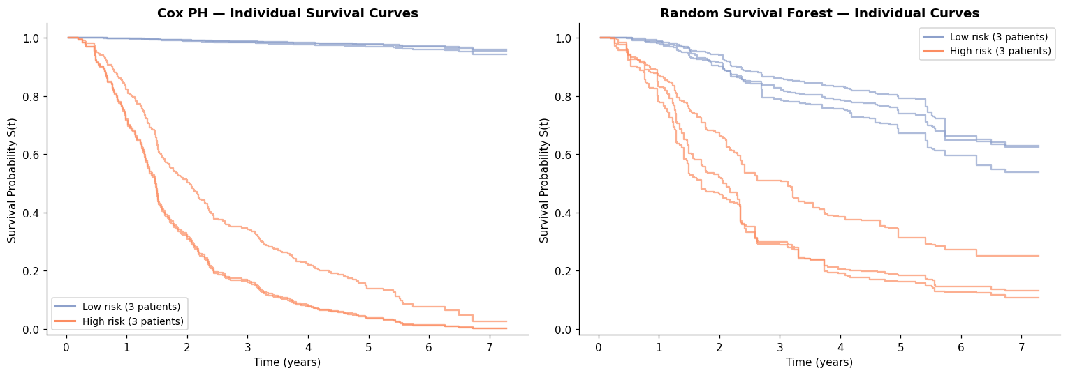
print("Notice: Cox curves have the same SHAPE (proportional hazards) but different LEVELS.")
print("RSF curves can have different shapes — the hazard ratio can change over time.")

Notice: Cox curves have the same SHAPE (proportional hazards) but different LEVELS.
RSF curves can have different shapes — the hazard ratio can change over time.

# ── Calibration-in-the-large: KM vs. average predicted survival ──────────────
fig, ax = plt.subplots(figsize=(8, 5))

# KM curve on validation set ("truth")
km_val_t, km_val_s = kaplan_meier_estimator(y_val['cens'], y_val['time'])
ax.step(km_val_t / 365.25, km_val_s, where='post', linewidth=2.5,
        color='black', label='Kaplan-Meier (observed)', linestyle='-')

# Average predicted survival from Cox
# Evaluate all individual curves on a common time grid
time_grid = np.linspace(0, y_val['time'].max(), 200)
cox_surv_matrix = np.array([sf(time_grid) for sf in surv_funcs_cox])
cox_mean_surv = cox_surv_matrix.mean(axis=0)
ax.plot(time_grid / 365.25, cox_mean_surv, linewidth=2,
        color=sns.color_palette('Set2')[0], label='Cox PH (mean predicted)')

# Average predicted survival from RSF
rsf_surv_matrix = np.array([sf(time_grid) for sf in surv_funcs_rsf])
rsf_mean_surv = rsf_surv_matrix.mean(axis=0)
ax.plot(time_grid / 365.25, rsf_mean_surv, linewidth=2,
        color=sns.color_palette('Set2')[2], label='RSF (mean predicted)')

ax.set_xlabel('Time (years)')
ax.set_ylabel('Survival Probability')
ax.set_title('Calibration-in-the-Large: Observed vs. Predicted Survival',
             fontweight='bold')
ax.set_ylim(-0.02, 1.05)
ax.legend(fontsize=10)
plt.tight_layout()
plt.show()

print("If the model is well-calibrated, the average predicted curve should")
print("closely track the Kaplan-Meier curve from the observed data.")

---------------------------------------------------------------------------
NameError                                 Traceback (most recent call last)
Cell In[15], line 5
      1 # ── Calibration-in-the-large: KM vs. average predicted survival ──────────────
      2 fig, ax = plt.subplots(figsize=(8, 5))
      3 
      4 # KM curve on validation set ("truth")
----> 5 km_val_t, km_val_s = kaplan_meier_estimator(y_val['cens'], y_val['time'])
      6 ax.step(km_val_t / 365.25, km_val_s, where='post', linewidth=2.5,
      7         color='black', label='Kaplan-Meier (observed)', linestyle='-')
      8 

NameError: name 'kaplan_meier_estimator' is not defined

🤔 Reflection 5.1 — Survival Curves in Clinical Practice

1. Two patients both have predicted median survival of 4 years. But one has a steep initial drop (high early risk, then a plateau) and the other has a gradual slope. How would you communicate this difference to a clinician? Why is the full survival curve more informative than a single risk score or median?

2. The Cox model’s individual survival curves have the same shape but different levels (because of the proportional hazards assumption). The RSF curves can cross each other. What does this mean about each model’s flexibility?

3. Look at the calibration plot. If the mean predicted curve is above the KM curve, the model is overestimating survival (underestimating risk). Is this more or less dangerous than the reverse?

---

Part 6 — Time-Dependent AUC & Clinical Utility

The C-index gives a single overall discrimination score. But clinically, we often care about prediction at specific time points: “How well can the model discriminate between patients who will recur within 1 year vs. those who won’t?”

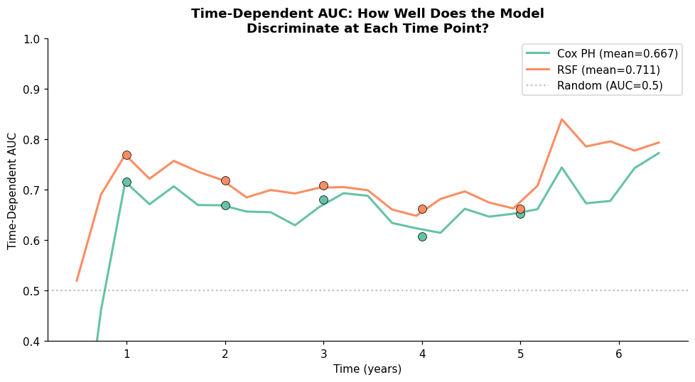
Time-dependent AUC at time \(t\) answers exactly this: it’s the AUC of the model for predicting whether the event occurs before or after time \(t\), accounting for censoring.

# ── Time-dependent AUC ───────────────────────────────────────────────────────
from sksurv.metrics import cumulative_dynamic_auc

# Evaluate at 1, 2, 3, 4, 5 year time points
eval_times = np.array([365.25, 730.5, 1095.75, 1461, 1826.25])  # 1-5 years in days
eval_years = eval_times / 365.25

# Filter to times within range of validation data
valid_mask = eval_times < y_val['time'].max()
eval_times_valid = eval_times[valid_mask]
eval_years_valid = eval_years[valid_mask]

# Cox PH
auc_cox, mean_auc_cox = cumulative_dynamic_auc(
    y_train, y_val, risk_cox_val, eval_times_valid)

# RSF
auc_rsf, mean_auc_rsf = cumulative_dynamic_auc(
    y_train, y_val, risk_rsf_val, eval_times_valid)

print(f"{'Time':>8s}  {'Cox AUC':>10s}  {'RSF AUC':>10s}")
print("─" * 32)
for yr, ac, ar in zip(eval_years_valid, auc_cox, auc_rsf):
    print(f"{yr:7.0f}y  {ac:10.4f}  {ar:10.4f}")
print("─" * 32)
print(f"{'Mean':>8s}  {mean_auc_cox:10.4f}  {mean_auc_rsf:10.4f}")

    Time     Cox AUC     RSF AUC
────────────────────────────────
      1y      0.7157      0.7691
      2y      0.6690      0.7190
      3y      0.6807      0.7091
      4y      0.6065      0.6614
      5y      0.6522      0.6628
────────────────────────────────
    Mean      0.6673      0.7110

# ── Visualize time-dependent AUC ─────────────────────────────────────────────
# Also compute on a finer grid for a smooth curve
fine_times = np.arange(180, y_val['time'].max() - 180, 90)  # every 3 months

auc_cox_fine, _ = cumulative_dynamic_auc(y_train, y_val, risk_cox_val, fine_times)
auc_rsf_fine, _ = cumulative_dynamic_auc(y_train, y_val, risk_rsf_val, fine_times)

fig, ax = plt.subplots(figsize=(9, 5))
ax.plot(fine_times / 365.25, auc_cox_fine, linewidth=2, label=f'Cox PH (mean={mean_auc_cox:.3f})')
ax.plot(fine_times / 365.25, auc_rsf_fine, linewidth=2, label=f'RSF (mean={mean_auc_rsf:.3f})')
ax.axhline(0.5, color='gray', linestyle=':', alpha=0.5, label='Random (AUC=0.5)')

# Mark the specific evaluation points
ax.scatter(eval_years_valid, auc_cox, s=60, zorder=5, color=sns.color_palette('Set2')[0],
           edgecolors='black', linewidth=0.5)
ax.scatter(eval_years_valid, auc_rsf, s=60, zorder=5, color=sns.color_palette('Set2')[1],
           edgecolors='black', linewidth=0.5)

ax.set_xlabel('Time (years)')
ax.set_ylabel('Time-Dependent AUC')
ax.set_title('Time-Dependent AUC: How Well Does the Model\nDiscriminate at Each Time Point?',
             fontweight='bold')
ax.legend(fontsize=10)
ax.set_ylim(0.4, 1.0)
plt.tight_layout()
plt.show()

🤔 Reflection 6.1 — Time-Dependent Discrimination

1. Suppose your model has C-index = 0.68 overall but time-AUC = 0.80 at 1 year and 0.58 at 5 years. What does this tell you about where the model is most useful? How would this change which clinical decisions you’d use it for?

2. Why might discrimination degrade at longer time horizons? (Hint: think about what information the features capture. Clinical features measured at diagnosis might predict short-term recurrence well but not long-term outcomes that depend on future treatment decisions, lifestyle changes, etc.)

3. At which time point(s) would you report the model’s performance to a clinical team? Would you choose the time point with the best AUC, or the most clinically relevant time horizon?

---

Part 7 — Final Test Set Evaluation

As always: evaluate on the test set once, using the model chosen on the validation set.

# ── Retrain on train + val ───────────────────────────────────────────────────
X_tv = np.vstack([X_train, X_val])
y_tv = np.concatenate([y_train, y_val])

final_cox = CoxPHSurvivalAnalysis(alpha=0.01)
final_cox.fit(X_tv, y_tv)

final_rsf = RandomSurvivalForest(n_estimators=100, max_depth=5, min_samples_leaf=10,
                                  random_state=42, n_jobs=-1)
final_rsf.fit(X_tv, y_tv)

# Risk scores on test set
risk_cox_test = final_cox.predict(X_test)
risk_rsf_test = final_rsf.predict(X_test)

# C-index
c_cox_test = concordance_index_censored(y_test['cens'], y_test['time'], risk_cox_test)[0]
c_rsf_test = concordance_index_censored(y_test['cens'], y_test['time'], risk_rsf_test)[0]

print("═" * 60)
print("  FINAL TEST SET EVALUATION")
print("═" * 60)
print(f"  Cox PH              — C-index: {c_cox_test:.4f}")
print(f"  Random Surv. Forest — C-index: {c_rsf_test:.4f}")

---------------------------------------------------------------------------
NameError                                 Traceback (most recent call last)
Cell In[18], line 17
     13 risk_cox_test = final_cox.predict(X_test)
     14 risk_rsf_test = final_rsf.predict(X_test)
     15 
     16 # C-index
---> 17 c_cox_test = concordance_index_censored(y_test['cens'], y_test['time'], risk_cox_test)[0]
     18 c_rsf_test = concordance_index_censored(y_test['cens'], y_test['time'], risk_rsf_test)[0]
     19 
     20 print("═" * 60)

NameError: name 'concordance_index_censored' is not defined

# ── Time-dependent AUC on test set ───────────────────────────────────────────
eval_times_test = eval_times[eval_times < y_test['time'].max()]
eval_years_test = eval_times_test / 365.25

auc_cox_test, mean_auc_cox_test = cumulative_dynamic_auc(
    y_tv, y_test, risk_cox_test, eval_times_test)
auc_rsf_test, mean_auc_rsf_test = cumulative_dynamic_auc(
    y_tv, y_test, risk_rsf_test, eval_times_test)

print(f"\n  Time-Dependent AUC (Test Set):")
print(f"  {'Time':>6s}  {'Cox':>8s}  {'RSF':>8s}")
print(f"  " + "─" * 26)
for yr, ac, ar in zip(eval_years_test, auc_cox_test, auc_rsf_test):
    print(f"  {yr:5.0f}y  {ac:8.4f}  {ar:8.4f}")
print(f"  " + "─" * 26)
print(f"  {'Mean':>6s}  {mean_auc_cox_test:8.4f}  {mean_auc_rsf_test:8.4f}")
print("═" * 60)

  Time-Dependent AUC (Test Set):
    Time       Cox       RSF
  ──────────────────────────
      1y    0.7226    0.7951
      2y    0.7625    0.8262
      3y    0.7239    0.7476
      4y    0.7203    0.7455
      5y    0.7348    0.7356
  ──────────────────────────
    Mean    0.7389    0.7861
════════════════════════════════════════════════════════════

# ── Final calibration plot ───────────────────────────────────────────────────
fig, ax = plt.subplots(figsize=(8, 5))

# KM on test set
km_test_t, km_test_s = kaplan_meier_estimator(y_test['cens'], y_test['time'])
ax.step(km_test_t / 365.25, km_test_s, where='post', linewidth=2.5,
        color='black', label='Kaplan-Meier (observed)')

# Mean predicted survival curves
surv_cox_test = final_cox.predict_survival_function(X_test)
surv_rsf_test = final_rsf.predict_survival_function(X_test)

tg = np.linspace(0, y_test['time'].max(), 200)
cox_test_matrix = np.array([sf(tg) for sf in surv_cox_test])
rsf_test_matrix = np.array([sf(tg) for sf in surv_rsf_test])

ax.plot(tg / 365.25, cox_test_matrix.mean(axis=0), linewidth=2,
        label=f'Cox PH (C={c_cox_test:.3f})', color=sns.color_palette('Set2')[0])
ax.plot(tg / 365.25, rsf_test_matrix.mean(axis=0), linewidth=2,
        label=f'RSF (C={c_rsf_test:.3f})', color=sns.color_palette('Set2')[2])

ax.set_xlabel('Time (years)')
ax.set_ylabel('Survival Probability')
ax.set_title('Test Set: Observed vs. Predicted Survival', fontweight='bold')
ax.set_ylim(-0.02, 1.05)
ax.legend(fontsize=10)
plt.tight_layout()
plt.show()

---------------------------------------------------------------------------
NameError                                 Traceback (most recent call last)
Cell In[20], line 5
      1 # ── Final calibration plot ───────────────────────────────────────────────────
      2 fig, ax = plt.subplots(figsize=(8, 5))
      3 
      4 # KM on test set
----> 5 km_test_t, km_test_s = kaplan_meier_estimator(y_test['cens'], y_test['time'])
      6 ax.step(km_test_t / 365.25, km_test_s, where='post', linewidth=2.5,
      7         color='black', label='Kaplan-Meier (observed)')
      8 

NameError: name 'kaplan_meier_estimator' is not defined

---

🤔 Final Reflection

A hospital wants to predict 30-day ICU readmission. They propose training a binary classifier: readmitted within 30 days — yes or no.

1. What information is lost by framing this as binary classification instead of a survival model? (Hint: consider two patients — one readmitted on day 2 and one readmitted on day 28. Consider a patient discharged 5 days ago who hasn’t been readmitted yet.)

2. Censoring in practice: Patients who are still within their 30-day window (discharge was recent) are right-censored: we know they haven’t been readmitted yet, but the 30-day window hasn’t closed. A binary classifier would have to either exclude these patients or guess. How does a survival model handle them?

3. Competing risks: Some patients are discharged to hospice and die within 30 days. They can’t be readmitted. This is a competing risk — an event that precludes the event of interest. How does ignoring competing risks bias the readmission prediction? (This is an advanced concept — just reason through the intuition.)

4. Connection to prior labs: How does the Cox partial likelihood loss compare to the losses in Labs 6–7? In what sense is it fundamentally different from cross-entropy (classification) and MSE (regression)?