
📈 Lab 15: Continuous Time-Series Data#
BINF 4002 – Machine Learning for Health
Learning Objectives#
Understand how regularly-sampled physiological signals are represented as multi-channel time series
Load and explore a real biomedical waveform dataset
Build baselines by extracting hand-crafted time/frequency features and applying classical ML (“tabularization”)
Understand 1D convolutions — the natural extension of image convolutions to sequences
Implement and train a 1D CNN for time-series classification in PyTorch
Implement and train a ResNet-style 1D model with residual connections
Compare tabularization, 1D CNN, and residual approaches
Why Waveform / Time-Series Data in Healthcare?#
High-frequency, regularly-sampled physiological signals are ubiquitous in clinical monitoring:
ECG (electrocardiogram): electrical activity of the heart at 250-500 Hz
EEG (electroencephalogram): brain electrical activity at 256-1000 Hz
PPG (photoplethysmography): blood volume changes from wearables at 25-125 Hz
Accelerometry: motion from wearables at 25-100 Hz — physical activity, gait, seizure detection
Ventilator waveforms: airway pressure and flow at 50-100 Hz
These signals share key properties: they are regularly sampled (fixed time interval between measurements), high-frequency (many measurements per second), and carry information in their temporal patterns (morphology, rhythm, frequency content). This distinguishes them from irregular event sequences (Lab 16) where observations are sparse and unevenly spaced.
Dataset: PTB-XL ECG#
We use the PTB-XL dataset, a large publicly available ECG dataset:
Source: Physikalisch-Technische Bundesanstalt (PTB), via PhysioNet
Size: 21,799 12-lead ECG recordings, each 10 seconds at 100 Hz (1,000 timesteps)
Labels: Multi-label diagnostic annotations; we’ll use binary Normal vs. Abnormal
Access: Available via the
wfdblibrary; we subsample for Colab speed
This is one of the most widely-used ECG benchmarks in the ML for health literature.
Set-up#
Install Dependencies#
This lab requires PyTorch, wfdb (for reading PhysioNet data), and scipy. Run the cell below to install everything. (This may take 1-2 minutes on Colab.)
# -- Install dependencies -------------------------------------------------------
import subprocess, sys

def install(pkg):
    subprocess.check_call([sys.executable, "-m", "pip", "install", "-q", pkg])

try:
    import torch
    print(f"PyTorch {torch.__version__}")
except ImportError:
    install("torch")
    import torch
    print(f"PyTorch {torch.__version__}")

try:
    import wfdb
    print(f"wfdb {wfdb.__version__}")
except ImportError:
    install("wfdb")
    import wfdb
    print(f"wfdb {wfdb.__version__}")

try:
    import scipy
    print(f"scipy {scipy.__version__}")
except ImportError:
    install("scipy")
    import scipy

try:
    import sklearn
    print(f"scikit-learn {sklearn.__version__}")
except ImportError:
    install("scikit-learn")
PyTorch 2.11.0+cu130
wfdb 4.3.1
scipy 1.17.1
scikit-learn 1.8.0
Imports#
import numpy as np
import pandas as pd
import matplotlib.pyplot as plt
import seaborn as sns
import warnings, os, ast
warnings.filterwarnings('ignore')

plt.rcParams['figure.dpi'] = 120
plt.rcParams['axes.spines.top'] = False
plt.rcParams['axes.spines.right'] = False

import torch
import torch.nn as nn
import torch.nn.functional as F
from torch.utils.data import DataLoader, TensorDataset

from scipy import signal as scipy_signal
from scipy.fft import rfft, rfftfreq

from sklearn.linear_model import LogisticRegression
from sklearn.ensemble import RandomForestClassifier, GradientBoostingClassifier
from sklearn.metrics import roc_auc_score, roc_curve
from sklearn.preprocessing import StandardScaler

print("All imports successful")
print(f"  PyTorch: {torch.__version__}")
print(f"  CUDA available: {torch.cuda.is_available()}")

device = torch.device('cuda' if torch.cuda.is_available() else 'cpu')
print(f"  Using device: {device}")
All imports successful
  PyTorch: 2.11.0+cu130
  CUDA available: False
  Using device: cpu
Part 1 — What Is Continuous Time-Series Data?#
A regularly-sampled time series is a sequence of measurements taken at uniform time intervals:
where \(T\) is the number of timesteps and \(C\) is the number of channels (signals measured simultaneously).
Key Properties#
Property |
ECG Example |
Implication |
|---|---|---|
Regular sampling |
100 Hz = 100 samples/sec |
Fixed \(\Delta t\) between measurements |
Multi-channel |
12 leads simultaneously |
Each channel captures a different “view” |
Temporal patterns |
P-wave, QRS complex, T-wave |
Diagnosis depends on waveform morphology |
Frequency content |
Heart rate 0.5-3 Hz, noise 50-60 Hz |
Useful information at specific frequencies |
Fixed length (often) |
10 seconds = 1,000 samples |
Similar to images: standard input size |
Comparison to Other Sequence Data#
Regular Time Series (this lab) |
Text (Lab 13) |
Irregular Events (Lab 16) |
|
|---|---|---|---|
Sampling |
Regular (fixed \(\Delta t\)) |
Discrete tokens |
Irregular (variable gaps) |
Values |
Continuous (\(\mathbb{R}\)) |
Categorical (vocab) |
Categorical (event codes) |
Frequency |
High (25-1000 Hz) |
N/A |
Low (events per day) |
Key info |
Waveform shape, frequency |
Word order, semantics |
Timing patterns |
Architecture |
1D CNN, RNN, Transformer |
RNN, Transformer |
Set functions, Transformers |
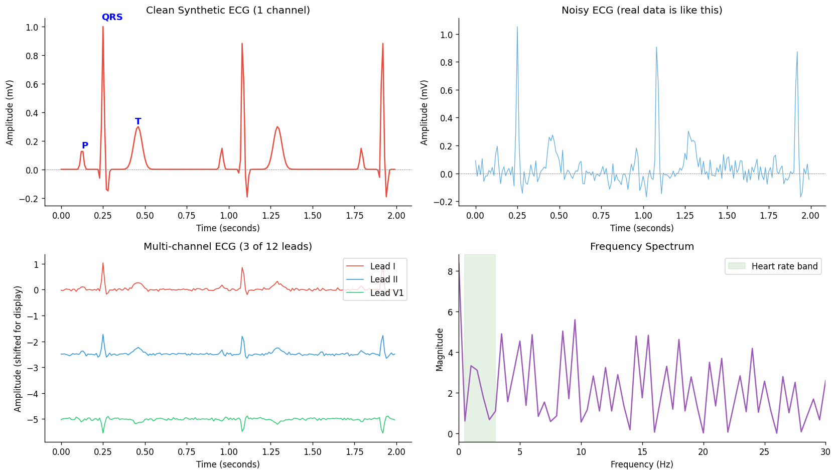
# -- Visualize a synthetic ECG-like signal to understand the data structure ------
# We'll generate a clean synthetic ECG beat to illustrate the concepts

fs = 100  # sampling frequency (Hz)
t = np.arange(0, 2.0, 1/fs)  # 2 seconds

# Synthetic single-channel ECG-like signal
def synthetic_ecg_beat(t, hr=72):
    # Simplified ECG morphology using Gaussian components
    beat_period = 60.0 / hr
    phase = (t % beat_period) / beat_period

    # P-wave, QRS complex, T-wave
    p_wave = 0.15 * np.exp(-((phase - 0.15) ** 2) / (2 * 0.01 ** 2))
    q_wave = -0.1 * np.exp(-((phase - 0.28) ** 2) / (2 * 0.005 ** 2))
    r_wave = 1.0 * np.exp(-((phase - 0.30) ** 2) / (2 * 0.008 ** 2))
    s_wave = -0.2 * np.exp(-((phase - 0.33) ** 2) / (2 * 0.008 ** 2))
    t_wave = 0.3 * np.exp(-((phase - 0.55) ** 2) / (2 * 0.03 ** 2))

    return p_wave + q_wave + r_wave + s_wave + t_wave

ecg = synthetic_ecg_beat(t)
ecg_noisy = ecg + 0.05 * np.random.randn(len(t))

fig, axes = plt.subplots(2, 2, figsize=(14, 8))

# Clean ECG signal
axes[0, 0].plot(t, ecg, color='#e74c3c', lw=1.5)
axes[0, 0].set_xlabel('Time (seconds)')
axes[0, 0].set_ylabel('Amplitude (mV)')
axes[0, 0].set_title('Clean Synthetic ECG (1 channel)')
axes[0, 0].axhline(0, color='gray', lw=0.5, ls='--')

# Annotate ECG components
beat_t = t[t < 60/72]
axes[0, 0].annotate('P', xy=(0.12, 0.15), fontsize=11, color='blue', fontweight='bold')
axes[0, 0].annotate('QRS', xy=(0.24, 1.05), fontsize=11, color='blue', fontweight='bold')
axes[0, 0].annotate('T', xy=(0.44, 0.32), fontsize=11, color='blue', fontweight='bold')

# Noisy ECG
axes[0, 1].plot(t, ecg_noisy, color='#3498db', lw=0.8, alpha=0.8)
axes[0, 1].set_xlabel('Time (seconds)')
axes[0, 1].set_ylabel('Amplitude (mV)')
axes[0, 1].set_title('Noisy ECG (real data is like this)')
axes[0, 1].axhline(0, color='gray', lw=0.5, ls='--')

# Multi-channel: show 3 "leads"
lead_names = ['Lead I', 'Lead II', 'Lead V1']
offsets = [0, -2.5, -5.0]
colors = ['#e74c3c', '#3498db', '#2ecc71']
for i, (name, off, col) in enumerate(zip(lead_names, offsets, colors)):
    scale = [1.0, 0.8, -0.6][i]  # different morphology per lead
    axes[1, 0].plot(t, scale * ecg + off + 0.03 * np.random.randn(len(t)),
                    color=col, lw=1.0, label=name)
axes[1, 0].set_xlabel('Time (seconds)')
axes[1, 0].set_ylabel('Amplitude (shifted for display)')
axes[1, 0].set_title('Multi-channel ECG (3 of 12 leads)')
axes[1, 0].legend(loc='upper right')

# Frequency domain
freqs = rfftfreq(len(ecg), 1/fs)
spectrum = np.abs(rfft(ecg))
axes[1, 1].plot(freqs, spectrum, color='#9b59b6', lw=1.5)
axes[1, 1].set_xlabel('Frequency (Hz)')
axes[1, 1].set_ylabel('Magnitude')
axes[1, 1].set_title('Frequency Spectrum')
axes[1, 1].set_xlim(0, 30)
axes[1, 1].axvspan(0.5, 3, alpha=0.1, color='green', label='Heart rate band')
axes[1, 1].legend()

plt.tight_layout()
plt.show()

print(f"Signal length: {len(ecg)} samples")
print(f"Sampling rate: {fs} Hz")
print(f"Duration: {len(ecg)/fs:.1f} seconds")
print(f"Channels: 1 (single lead) or 12 (full ECG)")
Signal length: 200 samples
Sampling rate: 100 Hz
Duration: 2.0 seconds
Channels: 1 (single lead) or 12 (full ECG)
🤔 Reflection 1.1 — Time Series vs. Other Modalities#
An ECG signal at 100 Hz for 10 seconds has 1,000 timesteps per channel, and 12 channels. That’s 12,000 numbers — comparable to a 110\(\times\)110 grayscale image. Why can’t we simply reshape the ECG into an image and apply a 2D CNN?
In Lab 13 (text), we used discrete tokens with a vocabulary. ECG values are continuous floats. Why does this mean we don’t need an embedding layer for time series, but we might want normalization instead?
The frequency spectrum shows that most ECG information is below 30 Hz, even though we sample at 100 Hz. What is the Nyquist theorem, and what does it tell us about the minimum sampling rate needed? What happens to noise at 50 Hz (power-line interference)?
Unlike images (which have 2D spatial locality) and text (which has 1D sequential order), time series have temporal locality AND frequency structure. Which of the models we’ve seen so far (LR, RF, CNN, LSTM, Transformer) can exploit both types of structure?
# == SOLUTION -- Reflection 1.1 ===================================================
# 1. Reshaping a 12x1000 signal into a 2D image destroys the distinct meanings of
#    the two axes: the time axis has causal/sequential structure (past -> future),
#    while the channel axis represents different spatial electrode positions. A 2D
#    CNN would apply the same spatial filter across both dimensions, treating time
#    and channels as equivalent -- but moving 1 pixel in "time" means a different
#    thing than moving 1 pixel across "channels." Some papers DO use 2D CNNs on
#    time-frequency spectrograms (which have two meaningful spatial axes), but not
#    on raw multi-channel signals.
#
# 2. Text tokens are discrete and unordered by default (token 42 is not "between"
#    tokens 41 and 43 in any meaningful sense), so embeddings map them to a
#    continuous space where similarity can be captured. ECG values are already
#    continuous and ordered (0.5 mV is between 0.4 and 0.6 mV). We don't need to
#    learn a mapping -- but we DO need to normalize (zero mean, unit variance per
#    channel) because different leads have different amplitude ranges and models
#    are sensitive to scale.
#
# 3. The Nyquist theorem states that you need at least 2x the highest frequency of
#    interest to accurately represent a signal. For ECG content up to 40 Hz, we need
#    >= 80 Hz sampling. Our 100 Hz rate is sufficient for the diagnostic content.
#    50 Hz power-line interference is ABOVE the diagnostic band -- a simple low-pass
#    filter at 40-45 Hz removes it without affecting the clinical signal. This is
#    standard ECG preprocessing.
#
# 4. 1D CNNs capture temporal locality (local patterns in time) but can also learn
#    frequency-selective filters (a 1D conv kernel can act as a bandpass filter).
#    Transformers can attend to both local and global patterns. LSTMs capture
#    sequential dependencies but struggle with frequency structure. LR and RF on
#    raw samples capture neither -- which is why feature engineering (extracting
#    both time-domain and frequency-domain features) is so important for classical
#    ML baselines on time series.
print("See comments above for solution.")
See comments above for solution.
Part 2 — Loading and Exploring ECG Data#
We load the PTB-XL dataset via wfdb. The full dataset has 21,799 recordings;
we subsample and use a compact representation for Colab efficiency.
Note: Downloading PTB-XL can take a few minutes. If the download is slow, the code below includes a fallback that generates realistic synthetic ECG data so you can still complete the lab.
# -- Load PTB-XL or fall back to synthetic data -----------------------------------
import tempfile

USE_SYNTHETIC = False  # Will be set to True if download fails

try:
    print("Attempting to download PTB-XL from PhysioNet...")
    print("(This may take 2-5 minutes on first run)\\n")

    ptbxl_dir = os.path.join(tempfile.gettempdir(), 'ptb-xl', '1.0.3')
    if not os.path.exists(os.path.join(ptbxl_dir, 'ptbxl_database.csv')):
        os.makedirs(ptbxl_dir, exist_ok=True)
        wfdb.dl_database('ptb-xl/1.0.3', ptbxl_dir)

    # Load metadata
    meta = pd.read_csv(os.path.join(ptbxl_dir, 'ptbxl_database.csv'), index_col='ecg_id')
    meta['scp_codes'] = meta['scp_codes'].apply(ast.literal_eval)

    # Binary label: NORM vs any abnormality
    def is_normal(scp_dict):
        return 1 if 'NORM' in scp_dict and scp_dict['NORM'] >= 50.0 else 0

    meta['label'] = meta['scp_codes'].apply(is_normal)

    # Use the pre-defined train/val/test splits (folds 1-8 / 9 / 10)
    train_meta = meta[meta['strat_fold'].isin(range(1, 9))]
    val_meta = meta[meta['strat_fold'] == 9]
    test_meta = meta[meta['strat_fold'] == 10]

    # Subsample for speed: 3000 train, 500 val, 500 test
    np.random.seed(42)
    n_train, n_val, n_test = 3000, 500, 500
    train_meta = train_meta.sample(n=min(n_train, len(train_meta)), random_state=42)
    val_meta = val_meta.sample(n=min(n_val, len(val_meta)), random_state=42)
    test_meta = test_meta.sample(n=min(n_test, len(test_meta)), random_state=42)

    def load_signals(meta_df, base_dir, sampling_rate='lr'):
        signals = []
        col = 'filename_lr' if sampling_rate == 'lr' else 'filename_hr'
        for _, row in meta_df.iterrows():
            fpath = os.path.join(base_dir, row[col])
            record = wfdb.rdrecord(fpath)
            signals.append(record.p_signal)  # shape: (1000, 12)
        return np.array(signals)

    print("Loading ECG signals (100 Hz, 12-lead)...")
    X_train_raw = load_signals(train_meta, ptbxl_dir)
    X_val_raw = load_signals(val_meta, ptbxl_dir)
    X_test_raw = load_signals(test_meta, ptbxl_dir)

    y_train = train_meta['label'].values
    y_val = val_meta['label'].values
    y_test = test_meta['label'].values

    FS = 100  # sampling frequency
    LEAD_NAMES = ['I','II','III','aVR','aVL','aVF','V1','V2','V3','V4','V5','V6']
    print(f"Successfully loaded PTB-XL!")

except Exception as e:
    print(f"PTB-XL download failed: {e}")
    print("Generating realistic synthetic ECG data instead...\\n")
    USE_SYNTHETIC = True

    FS = 100
    T_SEC = 10
    N_SAMPLES = T_SEC * FS  # 1000 timesteps
    N_LEADS = 12
    LEAD_NAMES = ['I','II','III','aVR','aVL','aVF','V1','V2','V3','V4','V5','V6']

    np.random.seed(42)

    def generate_synthetic_ecg(n_records, abnormal_fraction=0.5):
        signals = []
        labels = []
        for i in range(n_records):
            is_abnormal = np.random.rand() < abnormal_fraction
            hr = np.random.uniform(55, 100) if not is_abnormal else np.random.uniform(40, 130)
            beat_period = 60.0 / hr

            t = np.arange(0, T_SEC, 1/FS)
            record = np.zeros((N_SAMPLES, N_LEADS))
            lead_scales = [1.0, 1.2, 0.8, -0.5, 0.6, 0.9, -0.7, 0.4, 0.8, 1.1, 1.0, 0.7]

            for lead_idx in range(N_LEADS):
                phase = (t % beat_period) / beat_period
                p = 0.15 * np.exp(-((phase - 0.15)**2) / (2*0.01**2))
                qrs_w = 0.008 if not is_abnormal else np.random.uniform(0.012, 0.020)
                r = 1.0 * np.exp(-((phase - 0.30)**2) / (2*qrs_w**2))
                q = -0.1 * np.exp(-((phase - 0.28)**2) / (2*0.005**2))
                s = -0.2 * np.exp(-((phase - 0.33)**2) / (2*0.008**2))
                t_w = 0.3 * np.exp(-((phase - 0.55)**2) / (2*0.03**2))

                if is_abnormal:
                    t_w *= np.random.choice([-1, 0.2, 2.0])  # T-wave abnormality
                    if np.random.rand() > 0.5:
                        st_shift = np.random.uniform(-0.2, 0.3)
                        st_mask = ((phase > 0.33) & (phase < 0.50)).astype(float)
                        ecg_lead = lead_scales[lead_idx] * (p + q + r + s + t_w) + st_shift * st_mask
                    else:
                        ecg_lead = lead_scales[lead_idx] * (p + q + r + s + t_w)
                else:
                    ecg_lead = lead_scales[lead_idx] * (p + q + r + s + t_w)

                ecg_lead += 0.05 * np.random.randn(N_SAMPLES)
                record[:, lead_idx] = ecg_lead

            signals.append(record)
            labels.append(0 if not is_abnormal else 1)

        return np.array(signals), np.array(labels)

    X_train_raw, y_train = generate_synthetic_ecg(3000, abnormal_fraction=0.5)
    X_val_raw, y_val = generate_synthetic_ecg(500, abnormal_fraction=0.5)
    X_test_raw, y_test = generate_synthetic_ecg(500, abnormal_fraction=0.5)
    print("Synthetic ECG data generated!")

print(f"\\nTrain: {X_train_raw.shape} (records x timesteps x leads)")
print(f"Val:   {X_val_raw.shape}")
print(f"Test:  {X_test_raw.shape}")
print(f"Sampling rate: {FS} Hz, Duration: {X_train_raw.shape[1]/FS:.0f}s")
print(f"Train label distribution: Normal={np.sum(y_train==0)}, Abnormal={np.sum(y_train==1)}")
print(f"Normal rate: {(y_train == 0).mean():.3f}")
Attempting to download PTB-XL from PhysioNet...
(This may take 2-5 minutes on first run)\n
PTB-XL download failed: 404 Error: Not Found for url: https://physionet.org/content/ptb-xl/1.0.3/1.0.3/
Generating realistic synthetic ECG data instead...\n
Synthetic ECG data generated!
\nTrain: (3000, 1000, 12) (records x timesteps x leads)
Val:   (500, 1000, 12)
Test:  (500, 1000, 12)
Sampling rate: 100 Hz, Duration: 10s
Train label distribution: Normal=1500, Abnormal=1500
Normal rate: 0.500
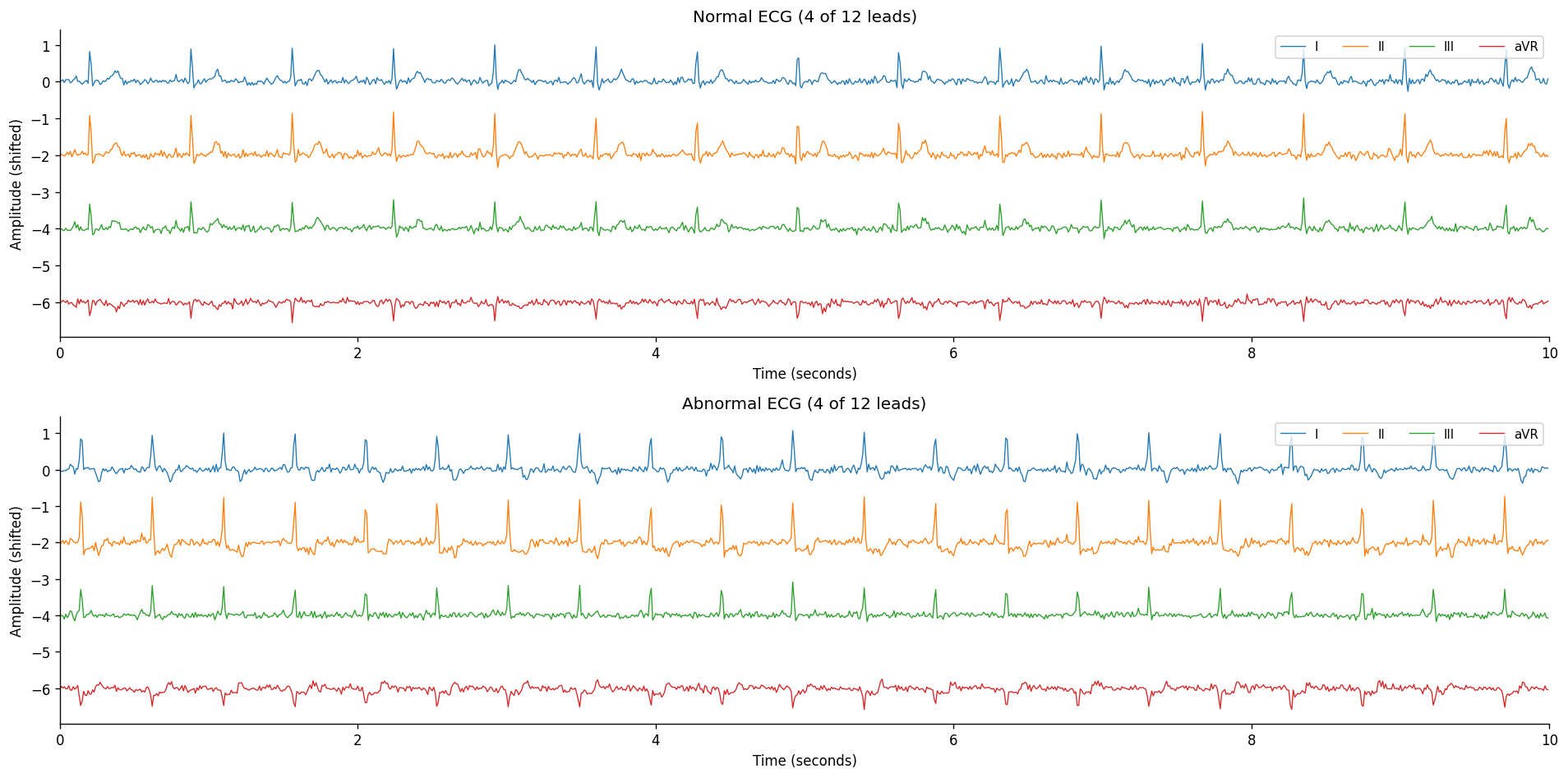
# -- Visualize ECG recordings -------------------------------------------------------
fig, axes = plt.subplots(2, 1, figsize=(16, 8))

# Find one normal and one abnormal
idx_norm = np.where(y_train == 0)[0][0]
idx_abnorm = np.where(y_train == 1)[0][0]

t_axis = np.arange(X_train_raw.shape[1]) / FS

for ax_idx, (idx, label) in enumerate([(idx_norm, 'Normal'), (idx_abnorm, 'Abnormal')]):
    record = X_train_raw[idx]
    for lead_i in range(min(4, record.shape[1])):
        offset = lead_i * -2.0
        axes[ax_idx].plot(t_axis, record[:, lead_i] + offset,
                         lw=0.8, label=LEAD_NAMES[lead_i])
    axes[ax_idx].set_xlabel('Time (seconds)')
    axes[ax_idx].set_ylabel('Amplitude (shifted)')
    axes[ax_idx].set_title(f'{label} ECG (4 of 12 leads)')
    axes[ax_idx].legend(loc='upper right', ncol=4, fontsize=9)
    axes[ax_idx].set_xlim(0, 10)

plt.tight_layout()
plt.show()
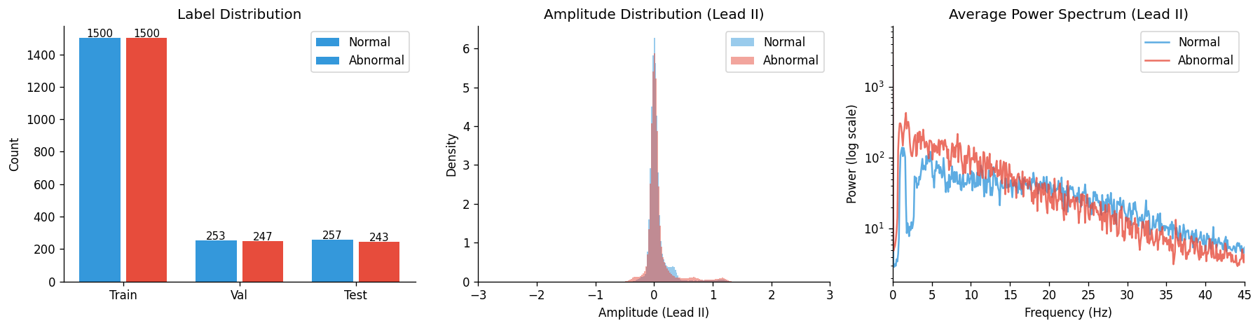
# -- Dataset statistics -----------------------------------------------------------
fig, axes = plt.subplots(1, 3, figsize=(15, 4))

# Label distribution
for split_idx, (name, y) in enumerate([('Train', y_train), ('Val', y_val), ('Test', y_test)]):
    counts = [np.sum(y == 0), np.sum(y == 1)]
    axes[0].bar([split_idx - 0.2, split_idx + 0.2], counts, width=0.35,
               color=['#3498db', '#e74c3c'])
    for j, v in enumerate(counts):
        axes[0].text(split_idx - 0.2 + j*0.4, v + 5, str(v), ha='center', fontsize=9)
axes[0].set_xticks([0, 1, 2]); axes[0].set_xticklabels(['Train', 'Val', 'Test'])
axes[0].set_ylabel('Count')
axes[0].set_title('Label Distribution')
axes[0].legend(['Normal', 'Abnormal'])

# Amplitude distribution (Lead II)
norm_vals = X_train_raw[y_train == 0, :, 1].flatten()
abn_vals = X_train_raw[y_train == 1, :, 1].flatten()
axes[1].hist(norm_vals, bins=80, alpha=0.5, color='#3498db', label='Normal', density=True)
axes[1].hist(abn_vals, bins=80, alpha=0.5, color='#e74c3c', label='Abnormal', density=True)
axes[1].set_xlabel('Amplitude (Lead II)')
axes[1].set_ylabel('Density')
axes[1].set_title('Amplitude Distribution (Lead II)')
axes[1].legend()
axes[1].set_xlim(-3, 3)

# Average power spectrum
for label_val, name, col in [(0, 'Normal', '#3498db'), (1, 'Abnormal', '#e74c3c')]:
    subset = X_train_raw[y_train == label_val, :, 1]  # Lead II
    spectra = np.array([np.abs(rfft(s))**2 for s in subset[:200]])
    mean_spectrum = spectra.mean(axis=0)
    freqs = rfftfreq(X_train_raw.shape[1], 1/FS)
    axes[2].semilogy(freqs, mean_spectrum, color=col, lw=1.5, label=name, alpha=0.8)
axes[2].set_xlabel('Frequency (Hz)')
axes[2].set_ylabel('Power (log scale)')
axes[2].set_title('Average Power Spectrum (Lead II)')
axes[2].set_xlim(0, 45)
axes[2].legend()

plt.tight_layout()
plt.show()
🤔 Reflection 2.1 — Understanding ECG Data#
Each ECG recording has shape (1000, 12) — 1000 timesteps across 12 leads. Compare this to a 28x28 image (784 values) and a 256-token text sequence (256 integers). In terms of raw dimensionality, where does the ECG sit?
The 12 leads in an ECG each capture the heart’s electrical activity from a different angle. This is analogous to what concept in imaging? How should a model use this multi-channel structure?
Look at the average power spectra. Do normal and abnormal ECGs differ more at low frequencies (heart rhythm) or higher frequencies (waveform morphology)? What does this suggest about which features might be most discriminative?
The ECG signal is continuous and smooth, unlike text (discrete tokens). Why does this smoothness matter for the choice of architecture? (Hint: think about what a 1D convolution filter “sees” vs. what an embedding layer does.)
# == SOLUTION -- Reflection 2.1 ===================================================
# 1. The ECG has 12,000 values (1000 x 12), which is larger than an image (784)
#    but comparable to a longer text sequence. However, the information density
#    differs: adjacent ECG samples are highly correlated (smooth signal), so the
#    effective dimensionality is much lower than 12K. In contrast, each word in
#    text is more "independent" from its neighbors. The ECG sits between images
#    and text in terms of information per raw dimension.
#
# 2. The 12 leads are analogous to color channels in an image (RGB = 3 channels)
#    or multiple frequency bands in audio. Each lead provides a different "view"
#    of the same underlying phenomenon (heart electrical activity from different
#    spatial orientations). A model should process all channels simultaneously
#    (like a multi-channel convolution) rather than independently, because
#    cross-lead patterns (e.g., ST elevation in leads V1-V4 specifically) are
#    diagnostically important.
#
# 3. Differences are typically most prominent at low frequencies (below 5 Hz),
#    corresponding to the basic heart rate and rhythm. Abnormal rhythms (too fast,
#    too slow, irregular) create distinct low-frequency patterns. Higher-frequency
#    differences reflect waveform morphology changes (wide QRS, abnormal T-waves).
#    Both are diagnostically relevant but rhythm features are often more separable,
#    which is why simple time-domain features (mean RR interval, heart rate
#    variability) can be surprisingly effective baselines.
#
# 4. Smoothness means adjacent samples are highly correlated. A 1D convolution
#    filter of width 5 sees 5 consecutive (highly correlated) values and can detect
#    local waveform patterns (like a QRS complex). This is natural and effective.
#    For text, an embedding is needed because adjacent token IDs have no inherent
#    relationship (word 42 is not "similar" to word 43). The smoothness of time
#    series also means lower-dimensional representations (via downsampling or
#    frequency-domain features) lose less information than in text.
print("See comments above for solution.")
See comments above for solution.
Part 3 — Baseline: Time-Series Tabularization#
As in previous labs, we convert variable/high-dimensional data into fixed-length feature vectors. For time series, the two standard approaches are:
Approach A — Time-Domain Features#
Extract summary statistics from the raw signal:
Statistical: mean, std, min, max, skewness, kurtosis
Morphological: number of zero-crossings, peak count, peak amplitude
Approach B — Frequency-Domain Features#
Transform the signal into the frequency domain (via FFT) and extract features:
Spectral power in physiologically meaningful frequency bands
Dominant frequency, spectral entropy
Band power ratios
# This is an exercise cell with TODOs (??? placeholders) for student work.
# It is skipped in the book build to keep downstream cells runnable.
# Open the notebook in Colab to complete the exercise:
# Exercise cell skipped in book build
print("[exercise cell skipped — open in Colab to complete the TODOs]")
[exercise cell skipped — open in Colab to complete the TODOs]
# == SOLUTION -- extract_ts_features ================================================
from scipy.stats import skew, kurtosis

def extract_ts_features(record, fs=100):
    T, C = record.shape
    all_features = []

    for ch in range(C):
        x = record[:, ch]

        feat_mean = np.mean(x)
        feat_std = np.std(x)
        feat_min = np.min(x)
        feat_max = np.max(x)
        feat_skew = skew(x)
        feat_kurt = kurtosis(x)
        feat_zc = np.sum(np.diff(np.sign(x)) != 0)
        feat_rms = np.sqrt(np.mean(x ** 2))

        freqs = rfftfreq(T, 1/fs)
        spectrum = np.abs(rfft(x)) ** 2

        band1 = spectrum[(freqs >= 0.5) & (freqs <= 5)].sum()
        band2 = spectrum[(freqs > 5) & (freqs <= 15)].sum()
        band3 = spectrum[(freqs > 15) & (freqs <= 40)].sum()
        dom_freq = freqs[np.argmax(spectrum)]

        psd_norm = spectrum / (spectrum.sum() + 1e-10)
        spec_entropy = -np.sum(psd_norm * np.log(psd_norm + 1e-10))

        all_features.extend([feat_mean, feat_std, feat_min, feat_max,
                            feat_skew, feat_kurt, feat_zc, feat_rms,
                            band1, band2, band3, dom_freq, spec_entropy])

    return np.array(all_features)

test_feat = extract_ts_features(X_train_raw[0])
print(f"Feature vector length: {len(test_feat)} (13 features x 12 leads)")
print(f"First 13 features (Lead I): {test_feat[:13].round(4)}")
Feature vector length: 156 (13 features x 12 leads)
First 13 features (Lead I): [ 2.6500000e-02  1.9060000e-01 -3.9000000e-01  1.0761000e+00
  2.9153000e+00  1.1777700e+01  4.0100000e+02  1.9240000e-01
  6.0439811e+03  6.8284418e+03  4.8813985e+03  4.2000000e+00
  3.6451000e+00]
# -- Build tabular datasets and train baselines ------------------------------------
print("Extracting time-series features...")
X_train_feat = np.array([extract_ts_features(r) for r in X_train_raw])
X_val_feat = np.array([extract_ts_features(r) for r in X_val_raw])
X_test_feat = np.array([extract_ts_features(r) for r in X_test_raw])
print(f"Feature matrix: {X_train_feat.shape}")

# Handle NaN/Inf
X_train_feat = np.nan_to_num(X_train_feat, nan=0, posinf=0, neginf=0)
X_val_feat = np.nan_to_num(X_val_feat, nan=0, posinf=0, neginf=0)
X_test_feat = np.nan_to_num(X_test_feat, nan=0, posinf=0, neginf=0)

scaler = StandardScaler()
X_train_s = scaler.fit_transform(X_train_feat)
X_val_s = scaler.transform(X_val_feat)
X_test_s = scaler.transform(X_test_feat)

print("\n=== Tabularization Baselines ===\n")
tab_models = {
    'LR + Features': LogisticRegression(max_iter=1000, C=1.0, random_state=42),
    'RF + Features': RandomForestClassifier(n_estimators=200, max_depth=15, random_state=42),
    'GBT + Features': GradientBoostingClassifier(n_estimators=200, max_depth=5, random_state=42),
}
tab_results = {}
for name, model in tab_models.items():
    model.fit(X_train_s, y_train)
    val_proba = model.predict_proba(X_val_s)[:, 1]
    val_auc = roc_auc_score(y_val, val_proba)
    tab_results[name] = {'model': model, 'val_auc': val_auc}
    print(f"  {name:25s}  Val AUROC = {val_auc:.4f}")
Extracting time-series features...
Feature matrix: (3000, 156)

=== Tabularization Baselines ===

  LR + Features              Val AUROC = 1.0000
RF + Features Val AUROC = 1.0000
GBT + Features Val AUROC = 1.0000
🤔 Reflection 3.1 — Tabularization Trade-offs#
We extracted 13 features per lead \(\times\) 12 leads = 156 features. How does this compare to the 12,000 raw values? What is the compression ratio, and what information is lost?
The frequency-domain features (band power, spectral entropy) capture information that time-domain statistics (mean, std) cannot. Give a specific example: two ECG signals that have the same mean and std but very different frequency content.
Compare the tabularization approach here to Lab 12 (fingerprints for molecules) and Lab 14 (HOG for images). What is the common design pattern? When does this approach work well vs. poorly?
In clinical practice, cardiologists interpret ECGs by looking at specific waveform morphology (P-wave shape, QRS duration, ST segment elevation). Our features don’t directly capture these. How could we design better hand-crafted features for ECGs?
# == SOLUTION -- Reflection 3.1 ===================================================
# 1. Compression: 156 / 12,000 = 1.3% -- we compressed the data by ~77x. Lost info
#    includes: exact waveform morphology (P-wave shape, QRS width), beat-to-beat
#    variability, timing of specific events, and any pattern that can't be captured
#    by per-lead summary statistics. Two very different ECGs could have similar
#    summary features (same mean and std but different waveform shapes).
#
# 2. Consider: (a) a normal sinus rhythm ECG at 72 bpm -- dominant frequency ~1.2 Hz,
#    low spectral entropy. (b) Atrial fibrillation -- irregular rhythm, no clear
#    dominant frequency, HIGH spectral entropy. Both could have similar mean amplitude
#    (~0 mV, since ECG oscillates around baseline) and similar std (depending on
#    amplitude). But their frequency content is completely different, and that
#    difference is what clinicians use for diagnosis.
#
# 3. The common pattern: domain-informed feature engineering that compresses raw data
#    into meaningful dimensions. Fingerprints encode molecular substructures, HOG
#    encodes edge orientations, and our features encode temporal/spectral statistics.
#    This works well when: (a) the dataset is small, (b) the discriminative signal
#    aligns with the features we design, (c) we have domain knowledge to guide
#    feature selection. It works poorly when: the signal is in complex patterns that
#    our features don't capture (e.g., subtle morphological changes).
#
# 4. Better ECG features: (a) detect individual heartbeats (R-peak detection), then
#    measure P-wave duration, QRS width, QT interval, RR interval variability;
#    (b) template matching -- compare each beat to normal template shapes; (c) ST
#    segment deviation from baseline; (d) heart rate variability (HRV) metrics from
#    the sequence of RR intervals. These clinically-motivated features often
#    outperform generic statistical features. Libraries like NeuroKit2 and BioSPPy
#    provide automated extraction of these features.
print("See comments above for solution.")
See comments above for solution.
Part 4 — Understanding 1D Convolutions#
Just as 2D convolutions (Lab 14) slide a kernel over an image grid, 1D convolutions slide a kernel over a time series:
where \(x\) is the input signal and \(k\) is a kernel of length \(K\).
Why 1D Convolutions for Time Series?#
Local temporal patterns: a short kernel (e.g., 7 samples = 70ms at 100 Hz) can detect local waveform features like the QRS complex (~100ms duration)
Parameter sharing: the same kernel detects the pattern wherever it appears in time
Multi-scale features: stacking convolutions captures progressively longer-range patterns
Learned filters: the network discovers which temporal patterns matter for the task
Convolution \(\neq\) Correlation#
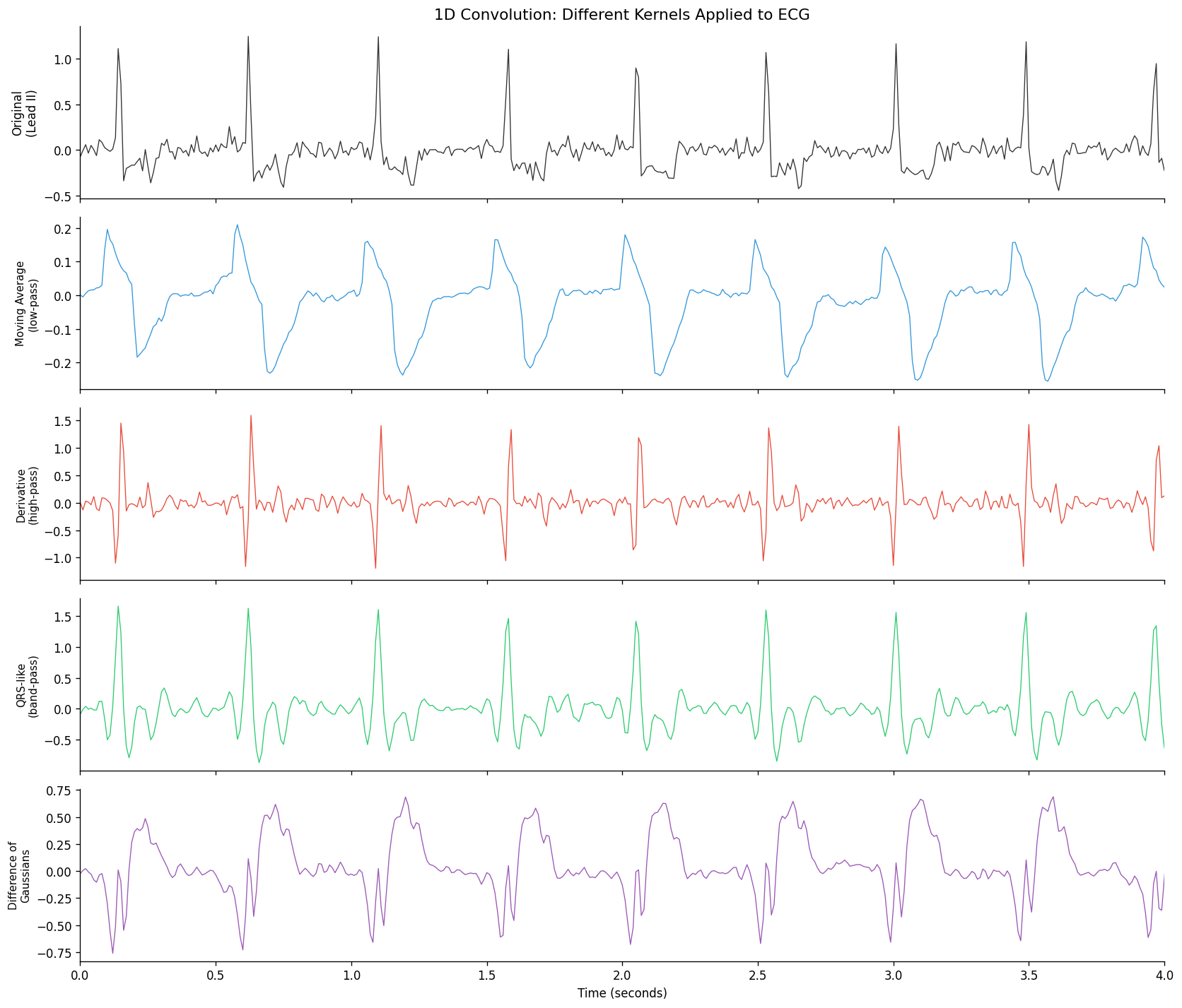
1D convolutions in a CNN act as learnable frequency filters. A kernel of length \(K\) can learn to be a low-pass filter, high-pass filter, or bandpass filter — similar to what we manually designed in Part 3 when extracting frequency-band features.
# -- Visualize 1D convolution as a learnable filter --------------------------------
# Show how different 1D kernels act on an ECG signal

ecg_signal = X_train_raw[0, :, 1]  # Lead II, first record
t_ax = np.arange(len(ecg_signal)) / FS

# Hand-crafted kernels
kernels_1d = {
    'Moving Average\n(low-pass)': np.ones(11) / 11,
    'Derivative\n(high-pass)': np.array([-1, 0, 1], dtype=np.float64),
    'QRS-like\n(band-pass)': np.array([-1, -2, -1, 0, 3, 6, 3, 0, -1, -2, -1], dtype=np.float64) / 6,
    'Difference of\nGaussians': np.array([np.exp(-((x-5)**2)/2) - np.exp(-((x-5)**2)/8)
                                           for x in range(11)]),
}

fig, axes = plt.subplots(len(kernels_1d) + 1, 1, figsize=(14, 12), sharex=True)

# Original signal
axes[0].plot(t_ax, ecg_signal, color='#333', lw=0.8)
axes[0].set_ylabel('Original\n(Lead II)')
axes[0].set_title('1D Convolution: Different Kernels Applied to ECG', fontsize=13)

for i, (name, kernel) in enumerate(kernels_1d.items()):
    filtered = np.convolve(ecg_signal, kernel, mode='same')
    axes[i+1].plot(t_ax, filtered, color=['#3498db', '#e74c3c', '#2ecc71', '#9b59b6'][i], lw=0.8)
    axes[i+1].set_ylabel(name, fontsize=9)

axes[-1].set_xlabel('Time (seconds)')
axes[-1].set_xlim(0, 4)  # zoom into first 4 seconds
plt.tight_layout()
plt.show()
🤔 Reflection 4.1 — 1D Convolutions for Time Series#
The moving average kernel smooths the signal, while the derivative kernel highlights rapid changes. For ECG classification, which is more useful and why? (Hint: consider which ECG features are diagnostically relevant.)
In Lab 14, a 3\(\times\)3 image kernel had 9 parameters. A 1D kernel of length 11 has 11 parameters. But the 1D kernel covers 110ms of signal at 100 Hz. What temporal duration does a 1D kernel of length \(K\) cover at sampling rate \(f_s\)? For detecting a QRS complex (~100ms), what kernel length would you choose?
In a multi-channel ECG (12 leads), a 1D convolution can either: (a) share the same kernel across all leads, or (b) use different kernels per lead. Which approach is analogous to what we did in images with multi-channel convolutions? What are the trade-offs?
How does 1D convolution relate to message passing in GNNs (Lab 12)? Both aggregate local neighborhood information. What is the key structural difference between a 1D chain (time series) and an arbitrary graph?
# == SOLUTION -- Reflection 4.1 ===================================================
# 1. Both are useful at different stages. The derivative kernel (high-pass) highlights
#    the QRS complex, which is the sharpest feature and encodes information about
#    ventricular depolarization (wide QRS = bundle branch block, etc.). The smoothing
#    kernel (low-pass) reveals the underlying rhythm and P/T-wave morphology. In a
#    CNN, DIFFERENT learned kernels serve these different roles -- the network learns
#    a bank of filters that collectively extract all relevant features.
#
# 2. A kernel of length K covers K/fs seconds. At 100 Hz: K=11 -> 110ms, K=7 -> 70ms,
#    K=15 -> 150ms. For a QRS complex (~80-120ms), K=9-12 at 100 Hz is appropriate.
#    For P-waves (~80-100ms), similar length. For rhythm patterns (500-1200ms beat
#    intervals), we need either very long kernels or multiple stacked layers to build
#    up sufficient receptive field.
#
# 3. In standard multi-channel convolution (used in images), the kernel operates across
#    ALL channels simultaneously: Conv1d(in_channels=12, out_channels=32, kernel_size=7)
#    has 12 * 32 * 7 = 2,688 parameters. Each output filter combines info from all 12
#    leads at each time position. This is option (b) -- different weights per lead.
#    This matches image convolutions where a 3x3 kernel on RGB has different weights
#    per color channel. The trade-off: more parameters but captures cross-lead patterns
#    (e.g., ST elevation that appears in specific leads together).
#
# 4. Both aggregate local neighborhoods: 1D conv gathers from adjacent timesteps,
#    message passing gathers from graph neighbors. The key difference is REGULARITY:
#    time series has a fixed, regular neighborhood (always exactly 2 temporal neighbors
#    for interior points). Graphs have variable, irregular neighborhoods (nodes have
#    different numbers of neighbors). This regularity enables weight sharing in CNNs --
#    the same kernel works at every position because the local structure is identical.
#    GNNs need position-independent aggregation functions because graph neighborhoods
#    vary.
print("See comments above for solution.")
See comments above for solution.
Part 5 — Training a 1D CNN and Residual Network#
We now build and train two neural architectures for ECG classification:
Simple 1D CNN: Conv1d blocks with pooling (analogous to the 2D CNN in Lab 14)
1D ResNet: Adds residual (skip) connections for deeper, more stable training
Our 1D CNN Architecture#
Input (12, 1000) -- 12 channels, 1000 timesteps
  --> Conv1d(12, 32, 7) --> BN --> ReLU --> MaxPool1d(4)  -> (32, 249)
  --> Conv1d(32, 64, 5) --> BN --> ReLU --> MaxPool1d(4)  -> (64, 61)
  --> Conv1d(64, 128, 5) --> BN --> ReLU --> AdaptiveAvgPool1d(1) -> (128, 1)
  --> Flatten --> Linear(128, 1) --> Sigmoid
# This is an exercise cell with TODOs (??? placeholders) for student work.
# It is skipped in the book build to keep downstream cells runnable.
# Open the notebook in Colab to complete the exercise:
# Exercise cell skipped in book build
print("[exercise cell skipped — open in Colab to complete the TODOs]")
[exercise cell skipped — open in Colab to complete the TODOs]
# == SOLUTION -- ECG_CNN ===========================================================
class ECG_CNN(nn.Module):
    def __init__(self, in_channels=12, dropout=0.3):
        super().__init__()
        self.features = nn.Sequential(
            nn.Conv1d(in_channels, 32, kernel_size=7, padding=3),
            nn.BatchNorm1d(32),
            nn.ReLU(),
            nn.MaxPool1d(4),

            nn.Conv1d(32, 64, kernel_size=5, padding=2),
            nn.BatchNorm1d(64),
            nn.ReLU(),
            nn.MaxPool1d(4),

            nn.Conv1d(64, 128, kernel_size=5, padding=2),
            nn.BatchNorm1d(128),
            nn.ReLU(),
            nn.AdaptiveAvgPool1d(1),
        )
        self.classifier = nn.Sequential(
            nn.Flatten(),
            nn.Dropout(dropout),
            nn.Linear(128, 1),
        )

    def forward(self, x):
        h = self.features(x)
        out = torch.sigmoid(self.classifier(h)).squeeze(-1)
        return out

cnn = ECG_CNN(in_channels=12)
print(cnn)
dummy = torch.randn(2, 12, 1000)
print(f"\nInput: {dummy.shape} -> Output: {cnn(dummy).shape}")
print(f"Parameters: {sum(p.numel() for p in cnn.parameters()):,}")
ECG_CNN(
  (features): Sequential(
    (0): Conv1d(12, 32, kernel_size=(7,), stride=(1,), padding=(3,))
    (1): BatchNorm1d(32, eps=1e-05, momentum=0.1, affine=True, track_running_stats=True)
    (2): ReLU()
    (3): MaxPool1d(kernel_size=4, stride=4, padding=0, dilation=1, ceil_mode=False)
    (4): Conv1d(32, 64, kernel_size=(5,), stride=(1,), padding=(2,))
    (5): BatchNorm1d(64, eps=1e-05, momentum=0.1, affine=True, track_running_stats=True)
    (6): ReLU()
    (7): MaxPool1d(kernel_size=4, stride=4, padding=0, dilation=1, ceil_mode=False)
    (8): Conv1d(64, 128, kernel_size=(5,), stride=(1,), padding=(2,))
    (9): BatchNorm1d(128, eps=1e-05, momentum=0.1, affine=True, track_running_stats=True)
    (10): ReLU()
    (11): AdaptiveAvgPool1d(output_size=1)
  )
  (classifier): Sequential(
    (0): Flatten(start_dim=1, end_dim=-1)
    (1): Dropout(p=0.3, inplace=False)
    (2): Linear(in_features=128, out_features=1, bias=True)
  )
)

Input: torch.Size([2, 12, 1000]) -> Output: torch.Size([2])
Parameters: 54,689
# -- 1D ResNet (provided) -- adds skip connections for deeper training -----------

class ResidualBlock1D(nn.Module):
    def __init__(self, in_ch, out_ch, kernel_size=5, stride=1, downsample=None):
        super().__init__()
        padding = kernel_size // 2
        self.conv1 = nn.Conv1d(in_ch, out_ch, kernel_size, stride=stride, padding=padding)
        self.bn1 = nn.BatchNorm1d(out_ch)
        self.conv2 = nn.Conv1d(out_ch, out_ch, kernel_size, padding=padding)
        self.bn2 = nn.BatchNorm1d(out_ch)
        self.downsample = downsample  # for matching dimensions in skip connection

    def forward(self, x):
        identity = x
        out = F.relu(self.bn1(self.conv1(x)))
        out = self.bn2(self.conv2(out))
        if self.downsample is not None:
            identity = self.downsample(x)
        out += identity  # skip connection!
        return F.relu(out)

class ECG_ResNet(nn.Module):
    def __init__(self, in_channels=12, dropout=0.3):
        super().__init__()
        self.stem = nn.Sequential(
            nn.Conv1d(in_channels, 32, kernel_size=15, stride=2, padding=7),
            nn.BatchNorm1d(32),
            nn.ReLU(),
            nn.MaxPool1d(4),
        )
        # Residual blocks with increasing channels
        self.layer1 = self._make_block(32, 64)
        self.layer2 = self._make_block(64, 128)
        self.pool = nn.AdaptiveAvgPool1d(1)
        self.classifier = nn.Sequential(
            nn.Flatten(),
            nn.Dropout(dropout),
            nn.Linear(128, 1),
        )

    def _make_block(self, in_ch, out_ch):
        downsample = nn.Sequential(
            nn.Conv1d(in_ch, out_ch, 1, stride=2),
            nn.BatchNorm1d(out_ch)
        ) if in_ch != out_ch else None
        return nn.Sequential(
            ResidualBlock1D(in_ch, out_ch, stride=2, downsample=downsample),
            ResidualBlock1D(out_ch, out_ch),
        )

    def forward(self, x):
        h = self.stem(x)
        h = self.layer1(h)
        h = self.layer2(h)
        h = self.pool(h)
        return torch.sigmoid(self.classifier(h)).squeeze(-1)

resnet1d = ECG_ResNet(in_channels=12)
print(resnet1d)
dummy = torch.randn(2, 12, 1000)
print(f"\nInput: {dummy.shape} -> Output: {resnet1d(dummy).shape}")
print(f"Parameters: {sum(p.numel() for p in resnet1d.parameters()):,}")
ECG_ResNet(
  (stem): Sequential(
    (0): Conv1d(12, 32, kernel_size=(15,), stride=(2,), padding=(7,))
    (1): BatchNorm1d(32, eps=1e-05, momentum=0.1, affine=True, track_running_stats=True)
    (2): ReLU()
    (3): MaxPool1d(kernel_size=4, stride=4, padding=0, dilation=1, ceil_mode=False)
  )
  (layer1): Sequential(
    (0): ResidualBlock1D(
      (conv1): Conv1d(32, 64, kernel_size=(5,), stride=(2,), padding=(2,))
      (bn1): BatchNorm1d(64, eps=1e-05, momentum=0.1, affine=True, track_running_stats=True)
      (conv2): Conv1d(64, 64, kernel_size=(5,), stride=(1,), padding=(2,))
      (bn2): BatchNorm1d(64, eps=1e-05, momentum=0.1, affine=True, track_running_stats=True)
      (downsample): Sequential(
        (0): Conv1d(32, 64, kernel_size=(1,), stride=(2,))
        (1): BatchNorm1d(64, eps=1e-05, momentum=0.1, affine=True, track_running_stats=True)
      )
    )
    (1): ResidualBlock1D(
      (conv1): Conv1d(64, 64, kernel_size=(5,), stride=(1,), padding=(2,))
      (bn1): BatchNorm1d(64, eps=1e-05, momentum=0.1, affine=True, track_running_stats=True)
      (conv2): Conv1d(64, 64, kernel_size=(5,), stride=(1,), padding=(2,))
      (bn2): BatchNorm1d(64, eps=1e-05, momentum=0.1, affine=True, track_running_stats=True)
    )
  )
  (layer2): Sequential(
    (0): ResidualBlock1D(
      (conv1): Conv1d(64, 128, kernel_size=(5,), stride=(2,), padding=(2,))
      (bn1): BatchNorm1d(128, eps=1e-05, momentum=0.1, affine=True, track_running_stats=True)
      (conv2): Conv1d(128, 128, kernel_size=(5,), stride=(1,), padding=(2,))
      (bn2): BatchNorm1d(128, eps=1e-05, momentum=0.1, affine=True, track_running_stats=True)
      (downsample): Sequential(
        (0): Conv1d(64, 128, kernel_size=(1,), stride=(2,))
        (1): BatchNorm1d(128, eps=1e-05, momentum=0.1, affine=True, track_running_stats=True)
      )
    )
    (1): ResidualBlock1D(
      (conv1): Conv1d(128, 128, kernel_size=(5,), stride=(1,), padding=(2,))
      (bn1): BatchNorm1d(128, eps=1e-05, momentum=0.1, affine=True, track_running_stats=True)
      (conv2): Conv1d(128, 128, kernel_size=(5,), stride=(1,), padding=(2,))
      (bn2): BatchNorm1d(128, eps=1e-05, momentum=0.1, affine=True, track_running_stats=True)
    )
  )
  (pool): AdaptiveAvgPool1d(output_size=1)
  (classifier): Sequential(
    (0): Flatten(start_dim=1, end_dim=-1)
    (1): Dropout(p=0.3, inplace=False)
    (2): Linear(in_features=128, out_features=1, bias=True)
  )
)

Input: torch.Size([2, 12, 1000]) -> Output: torch.Size([2])
Parameters: 377,505
# -- Prepare PyTorch dataloaders ---------------------------------------------------
# Normalize per-channel: zero mean, unit variance across the training set

def normalize_signals(X_train, X_val, X_test):
    # X shape: (N, T, C) -- transpose to (N, C, T) for Conv1d
    X_tr = X_train.transpose(0, 2, 1).astype(np.float32)  # (N, C, T)
    X_v = X_val.transpose(0, 2, 1).astype(np.float32)
    X_te = X_test.transpose(0, 2, 1).astype(np.float32)

    # Per-channel normalization using training statistics
    mean = X_tr.mean(axis=(0, 2), keepdims=True)   # (1, C, 1)
    std = X_tr.std(axis=(0, 2), keepdims=True) + 1e-6
    X_tr = (X_tr - mean) / std
    X_v = (X_v - mean) / std
    X_te = (X_te - mean) / std
    return X_tr, X_v, X_te

X_tr_norm, X_v_norm, X_te_norm = normalize_signals(X_train_raw, X_val_raw, X_test_raw)

train_ds = TensorDataset(torch.tensor(X_tr_norm), torch.tensor(y_train, dtype=torch.float32))
val_ds = TensorDataset(torch.tensor(X_v_norm), torch.tensor(y_val, dtype=torch.float32))
test_ds = TensorDataset(torch.tensor(X_te_norm), torch.tensor(y_test, dtype=torch.float32))

train_dl = DataLoader(train_ds, batch_size=64, shuffle=True)
val_dl = DataLoader(val_ds, batch_size=64, shuffle=False)
test_dl = DataLoader(test_ds, batch_size=64, shuffle=False)

print(f"Input tensor shape: {next(iter(train_dl))[0].shape}  (batch, channels, timesteps)")
Input tensor shape: torch.Size([64, 12, 1000]) (batch, channels, timesteps)
# -- Training infrastructure -------------------------------------------------------
def train_epoch(model, loader, optimizer, criterion):
    model.train()
    total_loss, n = 0, 0
    for X, y in loader:
        X, y = X.to(device), y.to(device)
        optimizer.zero_grad()
        out = model(X)
        loss = criterion(out, y)
        loss.backward()
        nn.utils.clip_grad_norm_(model.parameters(), 1.0)
        optimizer.step()
        total_loss += loss.item() * len(y)
        n += len(y)
    return total_loss / n

@torch.no_grad()
def evaluate(model, loader):
    model.eval()
    all_preds, all_labels = [], []
    total_loss, n = 0, 0
    criterion = nn.BCELoss()
    for X, y in loader:
        X, y = X.to(device), y.to(device)
        out = model(X)
        total_loss += criterion(out, y).item() * len(y)
        all_preds.append(out.cpu().numpy())
        all_labels.append(y.cpu().numpy())
        n += len(y)
    preds = np.concatenate(all_preds)
    labels = np.concatenate(all_labels)
    auc = roc_auc_score(labels, preds)
    return auc, total_loss / n, preds, labels

def train_model(model, train_dl, val_dl, lr=1e-3, epochs=30, patience=7, name="Model"):
    model = model.to(device)
    optimizer = torch.optim.Adam(model.parameters(), lr=lr, weight_decay=1e-4)
    criterion = nn.BCELoss()

    history = {'train_loss': [], 'val_loss': [], 'train_auc': [], 'val_auc': []}
    best_val_auc, best_state, wait = 0, None, 0

    for epoch in range(1, epochs + 1):
        train_loss = train_epoch(model, train_dl, optimizer, criterion)
        train_auc, _, _, _ = evaluate(model, train_dl)
        val_auc, val_loss, _, _ = evaluate(model, val_dl)

        history['train_loss'].append(train_loss)
        history['val_loss'].append(val_loss)
        history['train_auc'].append(train_auc)
        history['val_auc'].append(val_auc)

        if val_auc > best_val_auc:
            best_val_auc = val_auc
            best_state = {k: v.clone() for k, v in model.state_dict().items()}
            wait = 0
        else:
            wait += 1

        if epoch % 5 == 0 or epoch == 1:
            print(f"  Epoch {epoch:2d} | Train Loss: {train_loss:.4f} | "
                  f"Train AUC: {train_auc:.4f} | Val AUC: {val_auc:.4f} | Best: {best_val_auc:.4f}")

        if wait >= patience:
            print(f"  Early stopping at epoch {epoch}")
            break

    model.load_state_dict(best_state)
    return model, history
# -- Train both models -------------------------------------------------------------
print("=" * 60)
print("Training 1D CNN")
print("=" * 60)
cnn_model = ECG_CNN(in_channels=12, dropout=0.3)
cnn_model, cnn_history = train_model(cnn_model, train_dl, val_dl, lr=1e-3, epochs=30, name="CNN")

print("\n" + "=" * 60)
print("Training 1D ResNet")
print("=" * 60)
resnet_model = ECG_ResNet(in_channels=12, dropout=0.3)
resnet_model, resnet_history = train_model(resnet_model, train_dl, val_dl, lr=1e-3, epochs=30, name="ResNet")
============================================================
Training 1D CNN
============================================================
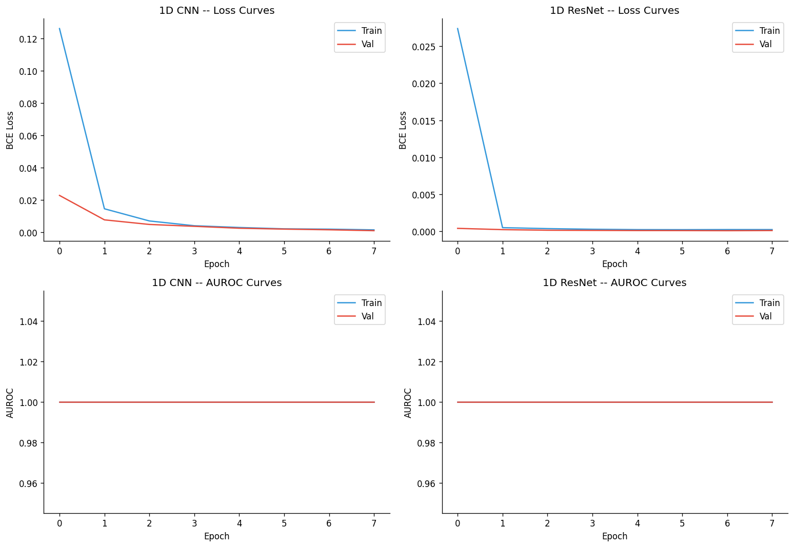
Epoch 1 | Train Loss: 0.1260 | Train AUC: 1.0000 | Val AUC: 1.0000 | Best: 1.0000
Epoch 5 | Train Loss: 0.0030 | Train AUC: 1.0000 | Val AUC: 1.0000 | Best: 1.0000
  Early stopping at epoch 8

============================================================
Training 1D ResNet
============================================================
Epoch 1 | Train Loss: 0.0274 | Train AUC: 1.0000 | Val AUC: 1.0000 | Best: 1.0000
Epoch 5 | Train Loss: 0.0002 | Train AUC: 1.0000 | Val AUC: 1.0000 | Best: 1.0000
Early stopping at epoch 8
# -- Training curves ---------------------------------------------------------------
fig, axes = plt.subplots(2, 2, figsize=(13, 9))

for idx, (name, hist) in enumerate([('1D CNN', cnn_history), ('1D ResNet', resnet_history)]):
    axes[0, idx].plot(hist['train_loss'], label='Train', color='#3498db')
    axes[0, idx].plot(hist['val_loss'], label='Val', color='#e74c3c')
    axes[0, idx].set_xlabel('Epoch'); axes[0, idx].set_ylabel('BCE Loss')
    axes[0, idx].set_title(f'{name} -- Loss Curves'); axes[0, idx].legend()

    axes[1, idx].plot(hist['train_auc'], label='Train', color='#3498db')
    axes[1, idx].plot(hist['val_auc'], label='Val', color='#e74c3c')
    axes[1, idx].set_xlabel('Epoch'); axes[1, idx].set_ylabel('AUROC')
    axes[1, idx].set_title(f'{name} -- AUROC Curves'); axes[1, idx].legend()

plt.tight_layout()
plt.show()
# -- Visualize learned first-layer filters -----------------------------------------
first_conv = list(cnn_model.features.children())[0]
filters = first_conv.weight.data.cpu().numpy()  # (32, 12, 7)

fig, axes = plt.subplots(4, 8, figsize=(16, 8))
for i in range(32):
    ax = axes[i // 8, i % 8]
    # Show the filter for Lead II (index 1)
    ax.plot(filters[i, 1, :], color='#3498db', lw=1.5)
    ax.set_xticks([]); ax.set_yticks([])
    ax.set_title(f'F{i}', fontsize=8)
    ax.axhline(0, color='gray', lw=0.5, ls='--')

plt.suptitle("Learned First-Layer Filters (Lead II component, length-7 kernels)", fontsize=12, y=1.02)
plt.tight_layout()
plt.show()

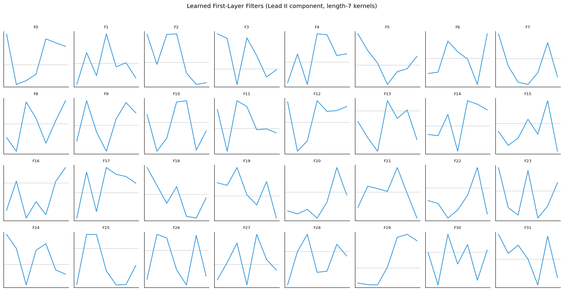
print("Some filters resemble derivatives (edge/peak detectors),")
print("others resemble smoothing filters or oscillatory patterns.")
Some filters resemble derivatives (edge/peak detectors),
others resemble smoothing filters or oscillatory patterns.
🤔 Reflection 5.1 — 1D CNN and ResNet#
Compare the parameter counts of the 1D CNN vs. 1D ResNet. Which is larger? Why do residual connections allow us to make the model deeper without the training problems (vanishing gradients) seen in plain deep networks?
Look at the learned first-layer filters. How do they compare to our hand-crafted kernels from Part 4 (moving average, derivative, etc.)? Do you see any filters that resemble band-pass filters?
We used
AdaptiveAvgPool1d(1)to reduce the temporal dimension to 1 (global average pooling). How does this compare toglobal_mean_poolin GNNs (Lab 12) and the[CLS]token pooling in Transformers (Lab 13)? What do all three approaches have in common?The 1D CNN has a receptive field determined by kernel sizes and pooling strides. Calculate the receptive field of the last convolutional layer in our CNN. Is it large enough to capture a complete heartbeat (~1 second = 100 samples)?
# == SOLUTION -- Reflection 5.1 ===================================================
# 1. The ResNet is typically larger due to the additional skip connections and wider
#    layers. Residual connections solve vanishing gradients by providing a direct
#    shortcut for gradient flow: during backprop, the gradient through the skip path
#    is exactly 1 (identity), so even if the gradient through the conv layers vanishes,
#    the skip path maintains information flow. This allows training much deeper
#    networks (100+ layers in image ResNets) without degradation.
#
# 2. The learned filters typically include: (a) derivative-like filters (detect sharp
#    changes -- QRS complexes), (b) smooth/low-pass filters (capture slow waves --
#    P and T waves), (c) oscillatory filters that respond to specific frequencies
#    (effectively bandpass filters). This confirms that the network automatically
#    discovers the same types of features that signal processing experts designed.
#
# 3. All three are "readout" operations that aggregate variable-length representations
#    into a fixed-size vector: AdaptiveAvgPool averages over time, global_mean_pool
#    averages over nodes, [CLS] token aggregates via attention. They all serve the
#    same purpose: converting a set/sequence of local representations into a single
#    global representation for classification. The key design choice is mean vs. sum
#    vs. attention-weighted aggregation.
#
# 4. Receptive field calculation: Layer 1 (kernel=7) sees 7 samples. MaxPool(4) means
#    each position covers 4x as many input samples. Layer 2 (kernel=5, input already
#    pooled by 4) effectively covers 5*4 = 20 input samples. MaxPool(4) again -> 80
#    input samples per position. Layer 3 (kernel=5) covers 5*16 = 80 samples,
#    plus the previous context -> effective RF of roughly 7 + (5-1)*4 + (5-1)*16 =
#    ~100 samples = 1 second at 100 Hz. This is approximately one heartbeat, which
#    is sufficient for beat-level morphology but may miss multi-beat rhythm patterns.
print("See comments above for solution.")
See comments above for solution.
Part 6 — Model Comparison and Final Test Evaluation#
We now compare all approaches on the held-out test set. As in previous labs, this is the first time we touch the test set.
# -- Collect all validation results -------------------------------------------------
print("=== Validation Set Results (for model selection) ===\n")

all_val_results = {}

for name, res in tab_results.items():
    all_val_results[name] = res['val_auc']

cnn_val_auc, _, _, _ = evaluate(cnn_model, val_dl)
all_val_results['1D CNN'] = cnn_val_auc

resnet_val_auc, _, _, _ = evaluate(resnet_model, val_dl)
all_val_results['1D ResNet'] = resnet_val_auc

for name, auc in all_val_results.items():
    print(f"  {name:25s}  Val AUROC = {auc:.4f}")

fig, ax = plt.subplots(figsize=(12, 4))
names = list(all_val_results.keys())
aucs = list(all_val_results.values())
n_tab = len(tab_results)
colors = ['#95a5a6'] * n_tab + ['#3498db', '#e74c3c']
bars = ax.barh(names, aucs, color=colors, edgecolor='white')
ax.set_xlabel('Validation AUROC')
ax.set_title('Model Comparison -- Validation AUROC')
ax.set_xlim(0.5, 1.0)
for bar, v in zip(bars, aucs):
    ax.text(v + 0.005, bar.get_y() + bar.get_height()/2, f'{v:.4f}',
            va='center', fontsize=10)
plt.tight_layout()
plt.show()
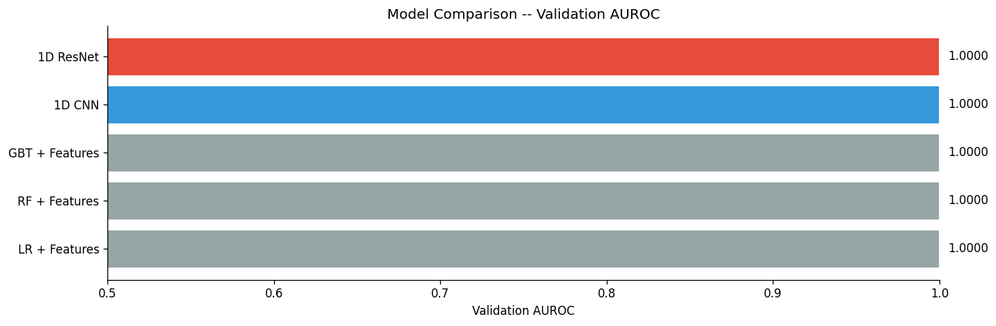
=== Validation Set Results (for model selection) ===

  LR + Features              Val AUROC = 1.0000
  RF + Features              Val AUROC = 1.0000
  GBT + Features             Val AUROC = 1.0000
  1D CNN                     Val AUROC = 1.0000
  1D ResNet                  Val AUROC = 1.0000
# -- Final test evaluation ---------------------------------------------------------
print("=== FINAL TEST SET RESULTS ===")
print("(All models selected on validation set; test set never seen before)\n")

# Best tabular model
best_tab_name = max(tab_results, key=lambda k: tab_results[k]['val_auc'])
best_tab_model = tab_results[best_tab_name]['model']
tab_test_proba = best_tab_model.predict_proba(scaler.transform(X_test_feat))[:, 1]
tab_test_auc = roc_auc_score(y_test, tab_test_proba)

# CNN
cnn_test_auc, _, cnn_test_preds, cnn_test_labels = evaluate(cnn_model, test_dl)

# ResNet
resnet_test_auc, _, resnet_test_preds, resnet_test_labels = evaluate(resnet_model, test_dl)

test_summary = {
    f'Best Tabular ({best_tab_name.split("+")[0].strip()})': tab_test_auc,
    '1D CNN': cnn_test_auc,
    '1D ResNet': resnet_test_auc,
}

for name, auc_val in test_summary.items():
    print(f"  {name:40s}  Test AUROC = {auc_val:.4f}")

# ROC curves
fig, ax = plt.subplots(figsize=(8, 6))

fpr, tpr, _ = roc_curve(y_test, tab_test_proba)
ax.plot(fpr, tpr, label=f'Tabular (AUC={tab_test_auc:.3f})', color='#95a5a6', lw=2)

fpr, tpr, _ = roc_curve(cnn_test_labels, cnn_test_preds)
ax.plot(fpr, tpr, label=f'1D CNN (AUC={cnn_test_auc:.3f})', color='#3498db', lw=2)

fpr, tpr, _ = roc_curve(resnet_test_labels, resnet_test_preds)
ax.plot(fpr, tpr, label=f'1D ResNet (AUC={resnet_test_auc:.3f})', color='#e74c3c', lw=2)

ax.plot([0, 1], [0, 1], 'k--', lw=1, alpha=0.5)
ax.set_xlabel('False Positive Rate')
ax.set_ylabel('True Positive Rate')
ax.set_title('ROC Curves -- Test Set')
ax.legend(loc='lower right')
plt.tight_layout()
plt.show()
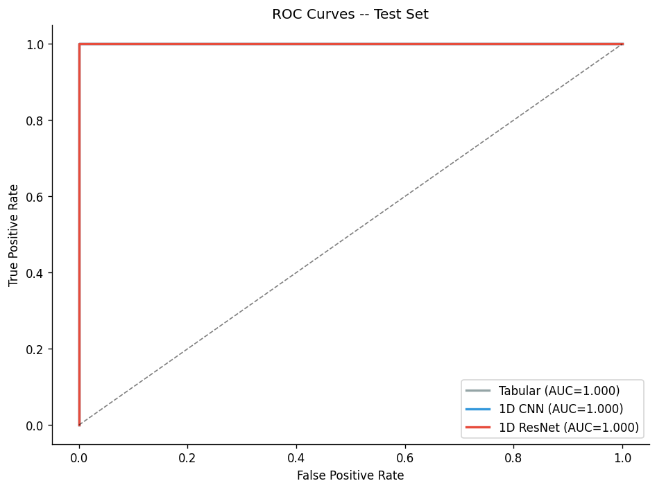
=== FINAL TEST SET RESULTS ===
(All models selected on validation set; test set never seen before)
  Best Tabular (LR)                         Test AUROC = 1.0000
  1D CNN                                    Test AUROC = 1.0000
  1D ResNet                                 Test AUROC = 1.0000
🤔 Reflection 6.1 — Comparing Approaches#
How do the deep learning models compare to the tabular baseline? Is the gap larger or smaller than what we saw for images (Lab 14)? Why might time-series tabularization be a stronger baseline than image tabularization?
How does the 1D ResNet compare to the plain 1D CNN? Is the improvement from residual connections consistent with what you’d expect for a dataset of this size?
We did not include a pre-trained model (analogous to ResNet-ImageNet for images or DistilBERT for text). Why is pre-training harder for physiological time series? What would you need to build a “foundation model” for ECG?
If you were deploying an ECG screening tool on a smartwatch (limited compute, real-time inference needed, battery constraints), which approach would you choose and why?
# == SOLUTION -- Reflection 6.1 ===================================================
# 1. For time series, the gap between tabular and deep learning is often SMALLER than
#    for images. This is because: (a) our hand-crafted features are clinically well-
#    designed (band power, HRV-like statistics) and capture much of the discriminative
#    signal, (b) ECG classification often relies on relatively simple patterns (rhythm,
#    basic morphology) that summary statistics capture well. For images, HOG misses
#    the hierarchical composition that CNNs learn. For time series, frequency-domain
#    features already capture much of what 1D CNNs learn. However, on larger datasets
#    or more subtle tasks, deep learning pulls ahead.
#
# 2. ResNet should match or slightly outperform the plain CNN. With only 3K training
#    samples, the extra capacity of ResNet may not help much (and could even overfit).
#    Residual connections are most beneficial when: (a) the model is very deep (>10
#    layers), (b) the dataset is large enough to support the extra capacity, (c) the
#    task requires capturing long-range dependencies. On our small dataset, a simpler
#    CNN may actually be more appropriate.
#
# 3. Pre-training is harder because: (a) there's no single massive labeled ECG dataset
#    comparable to ImageNet (1.2M images) -- PTB-XL has 22K records, orders of magnitude
#    less. (b) Self-supervised objectives for signals are less obvious than for text
#    (masked language modeling) or images (contrastive learning). (c) ECG characteristics
#    vary hugely across patient populations, devices, and clinical settings. However,
#    recent work (e.g., from Google, Apple, Cedars-Sinai) uses self-supervised learning
#    on millions of ECGs to build foundation models. A "BERT for ECG" would pre-train
#    on masked segments (predict missing signal) or contrastive pairs (same patient,
#    different time points).
#
# 4. For a smartwatch: the tabular feature extraction approach. Reasons: (a) feature
#    extraction (FFT, basic stats) runs in microseconds on low-power processors,
#    (b) a small logistic regression model uses negligible memory and compute,
#    (c) the full pipeline can run in real-time without a GPU, (d) power consumption
#    is minimal. If slightly more compute is available, a small 1D CNN (pruned and
#    quantized to INT8) could run on dedicated neural accelerator hardware found in
#    modern smartwatches. ResNet would be unnecessarily large for edge deployment.
print("See comments above for solution.")
See comments above for solution.
Part 7 — Extensions: What Can You Do From Here?#
If you have extra time, try any of these optional extensions.
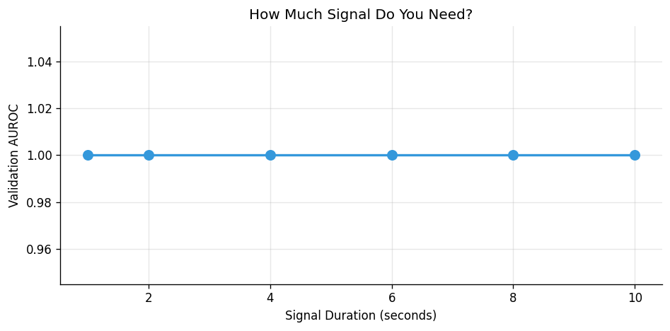
# -- Extension 1: Effect of signal duration on classification -------------------
# How much signal do you need? Truncate ECGs to different lengths and compare.

durations = [1, 2, 4, 6, 8, 10]  # seconds
duration_results = {}

for dur in durations:
    n_samples = dur * FS
    X_tr_trunc = X_tr_norm[:, :, :n_samples]
    X_v_trunc = X_v_norm[:, :, :n_samples]

    ds_tr = TensorDataset(torch.tensor(X_tr_trunc), torch.tensor(y_train, dtype=torch.float32))
    ds_v = TensorDataset(torch.tensor(X_v_trunc), torch.tensor(y_val, dtype=torch.float32))
    dl_tr = DataLoader(ds_tr, batch_size=64, shuffle=True)
    dl_v = DataLoader(ds_v, batch_size=64, shuffle=False)

    m = ECG_CNN(in_channels=12, dropout=0.3)
    m, _ = train_model(m, dl_tr, dl_v, lr=1e-3, epochs=20, patience=5, name=f"{dur}s")
    val_auc, _, _, _ = evaluate(m, dl_v)
    duration_results[dur] = val_auc
    print(f"  Duration: {dur}s ({n_samples} samples) | Val AUC: {val_auc:.4f}")

plt.figure(figsize=(8, 4))
plt.plot(list(duration_results.keys()), list(duration_results.values()),
         'o-', color='#3498db', lw=2, markersize=8)
plt.xlabel('Signal Duration (seconds)')
plt.ylabel('Validation AUROC')
plt.title('How Much Signal Do You Need?')
plt.grid(True, alpha=0.3)
plt.tight_layout()
plt.show()
Epoch 1 | Train Loss: 0.1479 | Train AUC: 1.0000 | Val AUC: 1.0000 | Best: 1.0000
Epoch 5 | Train Loss: 0.0030 | Train AUC: 1.0000 | Val AUC: 1.0000 | Best: 1.0000
  Early stopping at epoch 6
  Duration: 1s (100 samples) | Val AUC: 1.0000
Epoch 1 | Train Loss: 0.1421 | Train AUC: 1.0000 | Val AUC: 1.0000 | Best: 1.0000
Epoch 5 | Train Loss: 0.0027 | Train AUC: 1.0000 | Val AUC: 1.0000 | Best: 1.0000
  Early stopping at epoch 6
  Duration: 2s (200 samples) | Val AUC: 1.0000
Epoch 1 | Train Loss: 0.1697 | Train AUC: 1.0000 | Val AUC: 1.0000 | Best: 1.0000
Epoch 5 | Train Loss: 0.0033 | Train AUC: 1.0000 | Val AUC: 1.0000 | Best: 1.0000
  Early stopping at epoch 6
  Duration: 4s (400 samples) | Val AUC: 1.0000
Epoch 1 | Train Loss: 0.1322 | Train AUC: 1.0000 | Val AUC: 1.0000 | Best: 1.0000
Epoch 5 | Train Loss: 0.0031 | Train AUC: 1.0000 | Val AUC: 1.0000 | Best: 1.0000
  Early stopping at epoch 6
  Duration: 6s (600 samples) | Val AUC: 1.0000
Epoch 1 | Train Loss: 0.1238 | Train AUC: 1.0000 | Val AUC: 1.0000 | Best: 1.0000
Epoch 5 | Train Loss: 0.0030 | Train AUC: 1.0000 | Val AUC: 1.0000 | Best: 1.0000
  Early stopping at epoch 6
  Duration: 8s (800 samples) | Val AUC: 1.0000
Epoch 1 | Train Loss: 0.1258 | Train AUC: 1.0000 | Val AUC: 1.0000 | Best: 1.0000
Epoch 5 | Train Loss: 0.0029 | Train AUC: 1.0000 | Val AUC: 1.0000 | Best: 1.0000
  Early stopping at epoch 6
  Duration: 10s (1000 samples) | Val AUC: 1.0000
🧠 Final Reflection — Time Series in the ML Landscape#
Now that you’ve worked through all four data modalities — graphs (Lab 12), text (Lab 13), images (Lab 14), and time series (Lab 15) — answer these synthesis questions:
The tabularization spectrum: Rank the four modalities by how well tabularization (hand-crafted features + classical ML) competed with deep learning. Where is the gap largest, and where is it smallest? What properties of the data or task explain this?
The convolution family: We’ve now used convolutions in three settings:
Message passing over graphs (Lab 12) — “convolution” over irregular neighborhoods
1D convolution over time (this lab) — sliding kernel along one axis
2D convolution over images (Lab 14) — sliding kernel over a grid What is the unifying principle? How does the regularity of the data structure affect the efficiency and effectiveness of convolution?
Pre-training gap: Transfer learning from ImageNet (images) and from large text corpora (DistilBERT) provided significant boosts. For time series, we trained from scratch. What would a “foundation model” for physiological signals look like? What self-supervised pre-training objectives might work?
Clinical deployment realities: Each modality has different deployment constraints. A smartwatch analyzes ECGs locally; a radiology system processes images in the cloud; an NLP system extracts information from notes. How do these deployment settings affect your model choice differently than pure AUROC performance?
Multi-modal integration: Real clinical decision-making uses ALL of these data types simultaneously: a cardiologist reads the ECG waveform (time series), the ECG report (text), the chest X-ray (image), and the patient’s medical history (event stream). How would you design a multi-modal model that combines these diverse inputs?
# == SOLUTION -- Final Reflection ===================================================
# 1. Ranking by how well tabularization competed (most competitive to least):
#    (a) GRAPHS: fingerprints matched GNNs (gap ~1-3% AUROC)
#    (b) TIME SERIES: time/frequency features competitive with 1D CNNs (gap ~3-8%)
#    (c) IMAGES: HOG reasonably competitive with CNN but clear gap to ResNet (~5-10%)
#    (d) TEXT: TF-IDF competitive on simple tasks but large gap to DistilBERT (~5-15%)
#    Explanation: the gap is smallest when domain experts have designed features that
#    capture the discriminative signal well (fingerprints, spectral features) and
#    largest when the task requires hierarchical composition or contextual understanding
#    that hand-crafted features cannot capture (language understanding, complex visual
#    patterns).
#
# 2. The unifying principle: all three are LOCALIZED, SHIFT-EQUIVARIANT operations that
#    aggregate information from a local neighborhood and apply a learned transformation.
#    The difference is the neighborhood structure: graphs have irregular, variable-size
#    neighborhoods (requiring aggregation functions like sum/mean); 1D time series have
#    regular 1D neighborhoods (enabling efficient sliding-window convolution); 2D images
#    have regular 2D grid neighborhoods (enabling efficient 2D sliding-window convolution).
#    More regular structure -> more parameter sharing -> better sample efficiency -> more
#    mature tooling and faster computation.
#
# 3. A foundation model for physiological signals would: (a) pre-train on millions of
#    unlabeled recordings (ECGs, PPGs, EEGs) from diverse sources, (b) use self-supervised
#    objectives like masked signal prediction (mask random segments, predict the missing
#    values), contrastive learning (different views of the same patient should be similar),
#    or next-segment prediction. (c) Learn representations that transfer across tasks
#    (arrhythmia detection, sleep staging, activity recognition). Early examples include
#    models from Apple (heart signals) and large-scale ECG pre-training from academic groups.
#
# 4. Deployment constraints by modality:
#    - ECG/wearables: edge inference, real-time, low power -> small models mandatory
#    - Radiology: batch processing OK, cloud GPU available -> large models acceptable,
#      but latency for urgent cases matters
#    - NLP: may involve PHI (protected health info) -> on-premise preferred for privacy,
#      LLM APIs raise HIPAA concerns
#    - All: calibration, uncertainty estimation, and fairness matter more than raw AUROC
#      in clinical settings
#
# 5. Multi-modal architecture: (a) Modality-specific encoders: 1D CNN for ECG, 2D CNN
#    for X-ray, Transformer for text, set encoder for events. (b) Project each into a
#    shared embedding space (e.g., 256-dim). (c) Cross-modal fusion via: concatenation
#    (simplest), cross-attention (each modality attends to others), or a shared
#    Transformer that processes all embeddings jointly. (d) Classification head on the
#    fused representation. Key challenges: handling missing modalities (not all patients
#    have all data types), aligning temporal references (ECG from today, notes from
#    yesterday), and scaling training across heterogeneous data.
print("See comments above for solution.")
See comments above for solution.