🔬 Lab 7: Regression — MSE, MAE & Huber Loss

BINF 4002 – Machine Learning for Health

Every model in Labs 1–5 answered a binary question: malignant or benign? But many clinically important targets are continuous: tumor size in millimeters, blood pressure in mmHg, hospital length-of-stay in days, serum biomarker concentration. Predicting a continuous value instead of a class label is called regression, and it changes everything — the loss function, the model output, and how we evaluate performance.

Crucially, the shift from classification to regression is not a change of model architecture. The same linear model that performed logistic regression in Lab 1 can perform linear regression by swapping the loss function and removing the sigmoid. This lab is about that swap.

Learning Objectives

1. Understand regression as a change in loss function (MSE, MAE, Huber) rather than model

2. Implement MSE and MAE gradient computations by hand

3. Diagnose heteroscedasticity via residual plots

4. Appreciate clinical implications of point-estimate regression

Set-up

Upload data

⚠️ First, you need to upload the pre-processed data from lab0. If you have issues with running the first lab, you can also download the data here.

Once you have downloaded the data locally and started the runtime for this notebook, upload the file to this notebook via the “Files” menu.

import os

pkl_path = 'processed_data.pkl'
if os.path.exists(pkl_path):
    print("✅ Data File Found!")
else:
    raise FileNotFoundError(
        "processed_data.pkl not found! "
        "Make sure you have run Lab 0 (lab0_preprocessing.ipynb) in full and "
        "downloaded the output (or used the link above), and uploaded it here."
    )

✅ Data File Found!

Imports and Helper Functions

import numpy as np
import pandas as pd
import matplotlib.pyplot as plt
import matplotlib.gridspec as gridspec
import seaborn as sns
import pickle, warnings
from scipy import stats
warnings.filterwarnings('ignore')

plt.rcParams['figure.dpi'] = 110
plt.rcParams['axes.spines.top'] = False
plt.rcParams['axes.spines.right'] = False
sns.set_palette("Set2")

# ── Load data from Lab 0 ─────────────────────────────────────────────────────
with open('processed_data.pkl', 'rb') as f:
    d = pickle.load(f)

X_train_full = d['X_train']       # standardized, shape (341, 30)
X_val_full   = d['X_val']         # (114, 30)
X_test_full  = d['X_test']        # (114, 30)
feature_names_full = d['feature_names']
scaler = d['scaler']              # StandardScaler fit on training data

# Original binary labels — we'll use these as an INPUT feature
diagnosis_train = d['y_train']    # 0 = malignant, 1 = benign
diagnosis_val   = d['y_val']
diagnosis_test  = d['y_test']

print(f"Train: {X_train_full.shape}, Val: {X_val_full.shape}, Test: {X_test_full.shape}")
print(f"Features: {len(feature_names_full)}")

Train: (341, 30), Val: (114, 30), Test: (114, 30)
Features: 30

---

Part 1 — From Classification to Regression

We repurpose the Wisconsin Breast Cancer dataset for a regression task: predict the continuous feature mean radius (tumor size in mm) from the remaining features.

We drop mean radius, mean perimeter, and mean area from the inputs to remove trivially correlated variables (perimeter \(\approx 2\pi r\), area \(\approx \pi r^2\)). The original binary diagnosis label is included as an input — flipping the usual setup: “given we know the diagnosis, what tumor size do we expect?”

We work in original units (mm) for clinical interpretability, using the scaler from Lab 0 to invert the standardization on the target.

# ── Construct regression target and features ─────────────────────────────────
target_idx = feature_names_full.index('mean radius')

# Features to drop (trivially correlated with radius)
drop_names = ['mean radius', 'mean perimeter', 'mean area']
drop_idx = [feature_names_full.index(n) for n in drop_names]
keep_idx = [i for i in range(len(feature_names_full)) if i not in drop_idx]

# Extract target in ORIGINAL units (mm) for interpretability
target_mean  = scaler.mean_[target_idx]
target_scale = scaler.scale_[target_idx]

def to_original(z):
    """Convert standardized mean radius back to mm."""
    return z * target_scale + target_mean

def to_standardized(y):
    """Convert mm back to standardized units."""
    return (y - target_mean) / target_scale

y_train_mm = to_original(X_train_full[:, target_idx])
y_val_mm   = to_original(X_val_full[:, target_idx])
y_test_mm  = to_original(X_test_full[:, target_idx])

# Input features: remaining standardized features + binary diagnosis
X_train = np.column_stack([X_train_full[:, keep_idx], diagnosis_train])
X_val   = np.column_stack([X_val_full[:, keep_idx],   diagnosis_val])
X_test  = np.column_stack([X_test_full[:, keep_idx],  diagnosis_test])
feature_names = [feature_names_full[i] for i in keep_idx] + ['diagnosis (0=M, 1=B)']

# We'll work with original-scale targets for interpretability
y_train = y_train_mm
y_val   = y_val_mm
y_test  = y_test_mm

print(f"Input features: {X_train.shape[1]} ({len(keep_idx)} morphological + 1 diagnosis label)")
print(f"Target: mean radius (mm)")
print(f"\nTarget statistics (train):")
print(f"  Mean:   {y_train.mean():.2f} mm")
print(f"  Std:    {y_train.std():.2f} mm")
print(f"  Range:  [{y_train.min():.2f}, {y_train.max():.2f}] mm")
print(f"  Median: {np.median(y_train):.2f} mm")

Input features: 28 (27 morphological + 1 diagnosis label)
Target: mean radius (mm)

Target statistics (train):
  Mean:   14.07 mm
  Std:    3.46 mm
  Range:  [6.98, 25.22] mm
  Median: 13.27 mm

# ── Visualize the target distribution ────────────────────────────────────────
fig, axes = plt.subplots(1, 3, figsize=(15, 4))

# Histogram
axes[0].hist(y_train, bins=30, color=sns.color_palette('Set2')[0], edgecolor='white', alpha=0.8)
axes[0].axvline(y_train.mean(), color='red', linestyle='--', label=f'Mean={y_train.mean():.1f}')
axes[0].axvline(np.median(y_train), color='blue', linestyle='--', label=f'Median={np.median(y_train):.1f}')
axes[0].set_xlabel('Mean Radius (mm)')
axes[0].set_ylabel('Count')
axes[0].set_title('Target Distribution', fontweight='bold')
axes[0].legend(fontsize=9)

# By diagnosis
for diag, label, color in [(0, 'Malignant', sns.color_palette('Set2')[1]),
                            (1, 'Benign', sns.color_palette('Set2')[2])]:
    mask = diagnosis_train == diag
    axes[1].hist(y_train[mask], bins=20, alpha=0.6, color=color, edgecolor='white',
                 label=f'{label} (μ={y_train[mask].mean():.1f})')
axes[1].set_xlabel('Mean Radius (mm)')
axes[1].set_ylabel('Count')
axes[1].set_title('Radius by Diagnosis', fontweight='bold')
axes[1].legend(fontsize=9)

# Q-Q plot for normality check
stats.probplot(y_train, dist='norm', plot=axes[2])
axes[2].set_title('Q-Q Plot (Normality Check)', fontweight='bold')
axes[2].get_lines()[0].set_markersize(3)

plt.tight_layout()
plt.show()

print(f"Skewness: {stats.skew(y_train):.3f}  (positive → right-skewed)")
print(f"Kurtosis: {stats.kurtosis(y_train):.3f}")
print("\nThe distribution is right-skewed: most tumors are small, but some are quite large.")
print("Malignant tumors tend to be larger — diagnosis is a strong predictor of radius.")

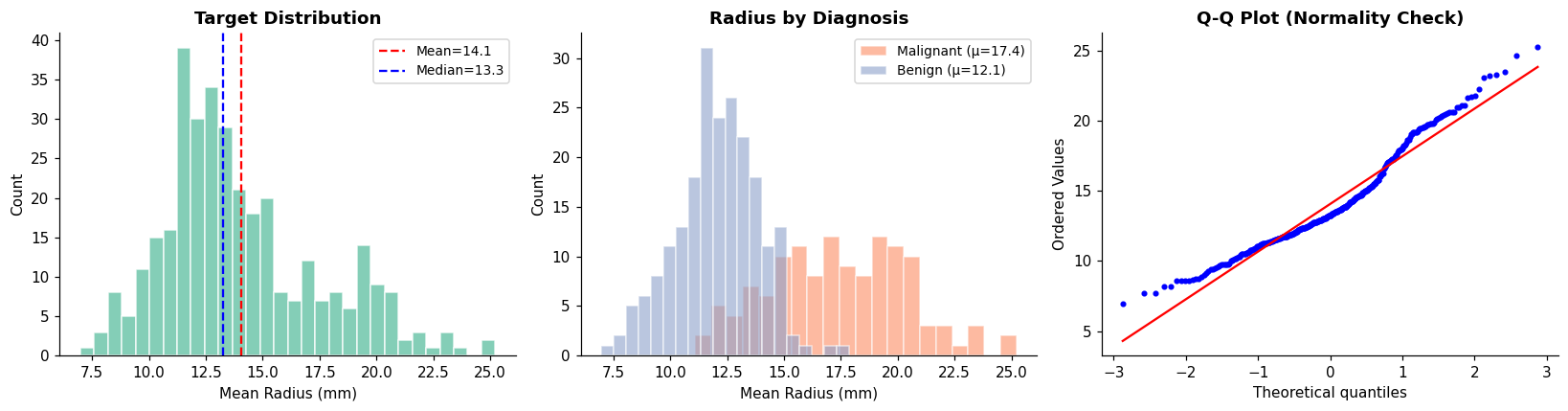
Skewness: 0.744  (positive → right-skewed)
Kurtosis: 0.079

The distribution is right-skewed: most tumors are small, but some are quite large.
Malignant tumors tend to be larger — diagnosis is a strong predictor of radius.

🤔 Reflection 1.1 — From Binary Labels to Continuous Targets

1. In Labs 1–5 we predicted a binary label and evaluated with accuracy, sensitivity, specificity, and AUROC. Now we predict a continuous value. Why can’t we use any of those metrics anymore? What would “accuracy” even mean for a continuous prediction?

2. The target is right-skewed (long tail of large tumors). What problems might this cause for a loss function like MSE that squares the errors? Will the model be disproportionately influenced by the few very large tumors?

3. We include the binary diagnosis label as an input feature. This flips the usual direction: normally we predict diagnosis from tumor measurements. Here we ask: “given the diagnosis, what size tumor do we expect?” When might this direction be clinically useful?

---

Part 2 — Implementing MSE & MAE from Scratch

The choice of loss function is the defining difference between regression problems. Each loss makes a different assumption about the error distribution:

Mean Squared Error (MSE): $\(\mathcal{L}_{\text{MSE}} = \frac{1}{n} \sum_{i=1}^{n} (y_i - \hat{y}_i)^2\)$

• Equivalent to maximum likelihood under Gaussian noise

• Penalizes large errors quadratically → sensitive to outliers

• Gradient: \(\frac{\partial \mathcal{L}}{\partial \hat{y}_i} = \frac{2}{n}(\hat{y}_i - y_i)\)

Mean Absolute Error (MAE): $\(\mathcal{L}_{\text{MAE}} = \frac{1}{n} \sum_{i=1}^{n} |y_i - \hat{y}_i|\)$

• Equivalent to maximum likelihood under Laplace noise

• Penalizes all errors linearly → robust to outliers

• Gradient: \(\frac{\partial \mathcal{L}}{\partial \hat{y}_i} = \frac{1}{n} \text{sign}(\hat{y}_i - y_i)\)

• Non-differentiable at \(\hat{y}_i = y_i\) (we use \(\text{sign}(0) = 0\) by convention)

def mse_loss_solution(y, y_hat):
    """Mean Squared Error."""
    return np.mean((y - y_hat) ** 2)

def mae_loss_solution(y, y_hat):
    """Mean Absolute Error."""
    return np.mean(np.abs(y - y_hat))

# Verify
y_check    = np.array([10.0, 15.0, 20.0, 25.0])
yhat_check = np.array([12.0, 14.0, 22.0, 20.0])
print(f"MSE: {mse_loss_solution(y_check, yhat_check):.4f} (expected: {np.mean((y_check - yhat_check)**2):.4f})")
print(f"MAE: {mae_loss_solution(y_check, yhat_check):.4f} (expected: {np.mean(np.abs(y_check - yhat_check)):.4f})")
print(f"Perfect MSE: {mse_loss_solution(y_check, y_check):.4f}")
print(f"Perfect MAE: {mae_loss_solution(y_check, y_check):.4f}")

MSE: 8.5000 (expected: 8.5000)
MAE: 2.5000 (expected: 2.5000)
Perfect MSE: 0.0000
Perfect MAE: 0.0000

def mse_grad_solution(y, y_hat):
    """Gradient of MSE w.r.t. y_hat."""
    return (2 / len(y)) * (y_hat - y)

def mae_grad_solution(y, y_hat):
    """Gradient of MAE w.r.t. y_hat."""
    return (1 / len(y)) * np.sign(y_hat - y)

# Verify shapes and values
y_demo = np.array([10.0, 15.0])
yhat_demo = np.array([12.0, 13.0])
print(f"MSE grad: {mse_grad_solution(y_demo, yhat_demo)}")
print(f"MAE grad: {mae_grad_solution(y_demo, yhat_demo)}")

MSE grad: [ 2. -2.]
MAE grad: [ 0.5 -0.5]

def train_linear_regression_solution(X_tr, y_tr, X_vl, y_vl, loss_fn, grad_fn,
                                       lr=0.01, n_epochs=500, label=''):
    """Train a linear model by gradient descent."""
    np.random.seed(42)
    n, d = X_tr.shape
    w = np.random.randn(d) * 0.01
    b = 0.0
    train_losses, val_losses = [], []

    for epoch in range(n_epochs):
        y_hat_tr = X_tr @ w + b
        loss_tr = loss_fn(y_tr, y_hat_tr)

        residual = grad_fn(y_tr, y_hat_tr)
        dw = X_tr.T @ residual
        db = residual.sum()

        w -= lr * dw
        b -= lr * db

        y_hat_vl = X_vl @ w + b
        loss_vl = loss_fn(y_vl, y_hat_vl)
        train_losses.append(loss_tr)
        val_losses.append(loss_vl)

    print(f"{label:8s} | Final train loss: {train_losses[-1]:.4f}, val loss: {val_losses[-1]:.4f}")
    return w, b, train_losses, val_losses

print("Solution function defined.")
print("Key insight: y_hat = X @ w + b (no sigmoid — this is regression).")
print("dw = X.T @ gradient, db = gradient.sum()")

Solution function defined.
Key insight: y_hat = X @ w + b (no sigmoid — this is regression).
dw = X.T @ gradient, db = gradient.sum()

# ── Plot loss curves ─────────────────────────────────────────────────────────
fig, axes = plt.subplots(1, 2, figsize=(13, 4.5))

axes[0].plot(tl_mse, label='Train', linewidth=2)
axes[0].plot(vl_mse, label='Validation', linewidth=2, linestyle='--')
axes[0].set_xlabel('Epoch')
axes[0].set_ylabel('MSE Loss (mm²)')
axes[0].set_title('MSE Training', fontweight='bold')
axes[0].legend()

axes[1].plot(tl_mae, label='Train', linewidth=2, color=sns.color_palette('Set2')[2])
axes[1].plot(vl_mae, label='Validation', linewidth=2, linestyle='--', color=sns.color_palette('Set2')[3])
axes[1].set_xlabel('Epoch')
axes[1].set_ylabel('MAE Loss (mm)')
axes[1].set_title('MAE Training', fontweight='bold')
axes[1].legend()

plt.tight_layout()
plt.show()

print("Note: MSE and MAE are in different units (mm² vs. mm), so their magnitudes")
print("are not directly comparable. RMSE = sqrt(MSE) converts to the same units as MAE.")

---------------------------------------------------------------------------
NameError                                 Traceback (most recent call last)
Cell In[8], line 4
      1 # ── Plot loss curves ─────────────────────────────────────────────────────────
      2 fig, axes = plt.subplots(1, 2, figsize=(13, 4.5))
      3 
----> 4 axes[0].plot(tl_mse, label='Train', linewidth=2)
      5 axes[0].plot(vl_mse, label='Validation', linewidth=2, linestyle='--')
      6 axes[0].set_xlabel('Epoch')
      7 axes[0].set_ylabel('MSE Loss (mm²)')

NameError: name 'tl_mse' is not defined

🤔 Reflection 2.1 — MSE vs. MAE

1. The MAE gradient is \(\frac{1}{n} \text{sign}(\hat{y}_i - y_i)\) — it doesn’t depend on the magnitude of the error, only its direction. What does this imply about how MAE treats outliers vs. MSE? If tumor measurements have occasional recording errors (e.g., “150 mm” instead of “15 mm”), which loss is more robust?

2. The MAE gradient is non-differentiable at \(\hat{y}_i = y_i\) (where the error is 0). Why does this cause the MAE loss curve to appear “noisier” than MSE during training? Does this matter in practice?

3. MSE-optimal predictions equal the conditional mean \(E[Y|X]\); MAE-optimal predictions equal the conditional median. For a right-skewed target like tumor size, these differ. Which is more clinically relevant — the mean or the median?

---

Part 3 — Huber Loss: The Best of Both Worlds?

The Huber loss combines MSE’s smooth gradient near zero with MAE’s robustness to outliers:

\[\begin{split}L_\delta(r) = \begin{cases} \frac{1}{2} r^2 & \text{if } |r| \leq \delta \\ \delta \left(|r| - \frac{1}{2}\delta\right) & \text{otherwise} \end{cases}\end{split}\]

where \(r = \hat{y} - y\) is the residual and \(\delta > 0\) is a tunable threshold.

• When \(\delta \to \infty\): Huber behaves like MSE (quadratic everywhere)

• When \(\delta \to 0\): Huber behaves like MAE (linear everywhere)

• The transition at \(|r| = \delta\) is smooth (continuous first derivative)

def huber_loss_solution(y, y_hat, delta=1.0):
    """Huber loss with threshold delta."""
    r = y_hat - y
    abs_r = np.abs(r)
    loss = np.where(abs_r <= delta, 0.5 * r**2, delta * (abs_r - 0.5 * delta))
    return np.mean(loss)

def huber_grad_solution(y, y_hat, delta=1.0):
    """Gradient of Huber loss w.r.t. y_hat."""
    r = y_hat - y
    abs_r = np.abs(r)
    grad = np.where(abs_r <= delta, r, delta * np.sign(r))
    return grad / len(y)

# Verify
y_small = np.array([10.0, 10.0])
yhat_small = np.array([10.3, 9.8])
print(f"Small errors — Huber(δ=1): {huber_loss_solution(y_small, yhat_small, delta=1.0):.6f}")
print(f"              0.5 * MSE:   {0.5 * mse_loss_solution(y_small, yhat_small):.6f}")

y_big = np.array([10.0])
yhat_big = np.array([20.0])
print(f"Large error — Huber(δ=1): {huber_loss_solution(y_big, yhat_big, delta=1.0):.4f}")
print(f"              δ(|r|-δ/2): {1.0 * (10.0 - 0.5):.4f}")

Small errors — Huber(δ=1): 0.032500
              0.5 * MSE:   0.032500
Large error — Huber(δ=1): 9.5000
              δ(|r|-δ/2): 9.5000

# ── Visualize how Huber interpolates between MSE and MAE ─────────────────────
errors = np.linspace(-6, 6, 300)

fig, axes = plt.subplots(1, 2, figsize=(13, 4.5))

# Loss curves for different delta values
axes[0].plot(errors, errors**2, 'k:', linewidth=1.5, alpha=0.5, label='MSE: $e^2$')
axes[0].plot(errors, np.abs(errors), 'k--', linewidth=1.5, alpha=0.5, label='MAE: $|e|$')

deltas = [0.5, 1.0, 2.0, 4.0]
colors = sns.color_palette('viridis', len(deltas))
for delta, color in zip(deltas, colors):
    abs_e = np.abs(errors)
    huber_vals = np.where(abs_e <= delta, 0.5 * errors**2, delta * (abs_e - 0.5 * delta))
    axes[0].plot(errors, huber_vals, color=color, linewidth=2, label=f'Huber δ={delta}')

axes[0].set_xlabel('Error ($\hat{y} - y$)')
axes[0].set_ylabel('Loss (single sample)')
axes[0].set_title('Huber Loss for Various δ', fontweight='bold')
axes[0].legend(fontsize=8, loc='upper center')
axes[0].set_ylim(-0.5, 20)

# Gradient curves
axes[1].plot(errors, 2 * errors, 'k:', linewidth=1.5, alpha=0.5, label='MSE grad: $2e$')
axes[1].plot(errors, np.sign(errors), 'k--', linewidth=1.5, alpha=0.5, label='MAE grad: sign($e$)')

for delta, color in zip(deltas, colors):
    abs_e = np.abs(errors)
    huber_g = np.where(abs_e <= delta, errors, delta * np.sign(errors))
    axes[1].plot(errors, huber_g, color=color, linewidth=2, label=f'Huber δ={delta}')

axes[1].set_xlabel('Error ($\hat{y} - y$)')
axes[1].set_ylabel('Gradient')
axes[1].set_title('Huber Gradient for Various δ', fontweight='bold')
axes[1].legend(fontsize=8, loc='upper left')
axes[1].axhline(0, color='gray', linewidth=0.5)

plt.tight_layout()
plt.show()

print("Small δ: Huber quickly transitions to linear → more robust to outliers.")
print("Large δ: Huber stays quadratic longer → more like MSE.")

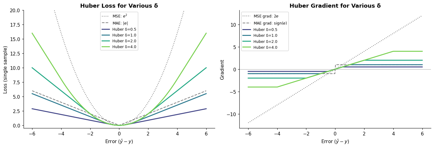
Small δ: Huber quickly transitions to linear → more robust to outliers.
Large δ: Huber stays quadratic longer → more like MSE.

# ── Sweep δ values and compare validation performance ────────────────────────
deltas_sweep = [0.1, 0.5, 1.0, 2.0, 5.0, 10.0, 50.0]
huber_results = []

for delta in deltas_sweep:
    # Create loss/grad functions with this delta
    loss_fn = lambda y, yh, d=delta: huber_loss(y, yh, delta=d)
    grad_fn = lambda y, yh, d=delta: huber_grad(y, yh, delta=d)

    w_h, b_h, tl_h, vl_h = train_linear_regression(
        X_train, y_train, X_val, y_val,
        loss_fn, grad_fn, lr=0.001, n_epochs=1000, label=f'δ={delta}')

    # Evaluate with MSE and MAE (universal metrics)
    yhat_val = X_val @ w_h + b_h
    huber_results.append({
        'delta': delta,
        'val_mse': mse_loss(y_val, yhat_val),
        'val_mae': mae_loss(y_val, yhat_val),
        'val_rmse': np.sqrt(mse_loss(y_val, yhat_val))
    })

hr_df = pd.DataFrame(huber_results)
print("\n" + hr_df.to_string(index=False, float_format='%.4f'))

---------------------------------------------------------------------------
NameError                                 Traceback (most recent call last)
Cell In[11], line 10
      6     # Create loss/grad functions with this delta
      7     loss_fn = lambda y, yh, d=delta: huber_loss(y, yh, delta=d)
      8     grad_fn = lambda y, yh, d=delta: huber_grad(y, yh, delta=d)
      9 
---> 10     w_h, b_h, tl_h, vl_h = train_linear_regression(
     11         X_train, y_train, X_val, y_val,
     12         loss_fn, grad_fn, lr=0.001, n_epochs=1000, label=f'δ={delta}')
     13 

NameError: name 'train_linear_regression' is not defined

🤔 Reflection 3.1 — Choosing δ

1. How would you choose \(\delta\) in practice? One approach: set \(\delta\) to the expected magnitude of typical measurement noise, so errors within normal noise get quadratic treatment while outliers get linear treatment. If tumor radius measurements have \(\pm 0.5\) mm precision, what \(\delta\) would you suggest (in the original mm scale)?

2. Look at the sweep results. As \(\delta\) increases, the Huber model approaches the MSE model. As \(\delta\) decreases, it approaches MAE. Is there a clear “best” \(\delta\), or is the difference small? What does this tell you about the outlier situation in this dataset?

3. Could you use cross-validation to select \(\delta\)? What metric would you optimize?

---

Part 4 — Residual Diagnostics

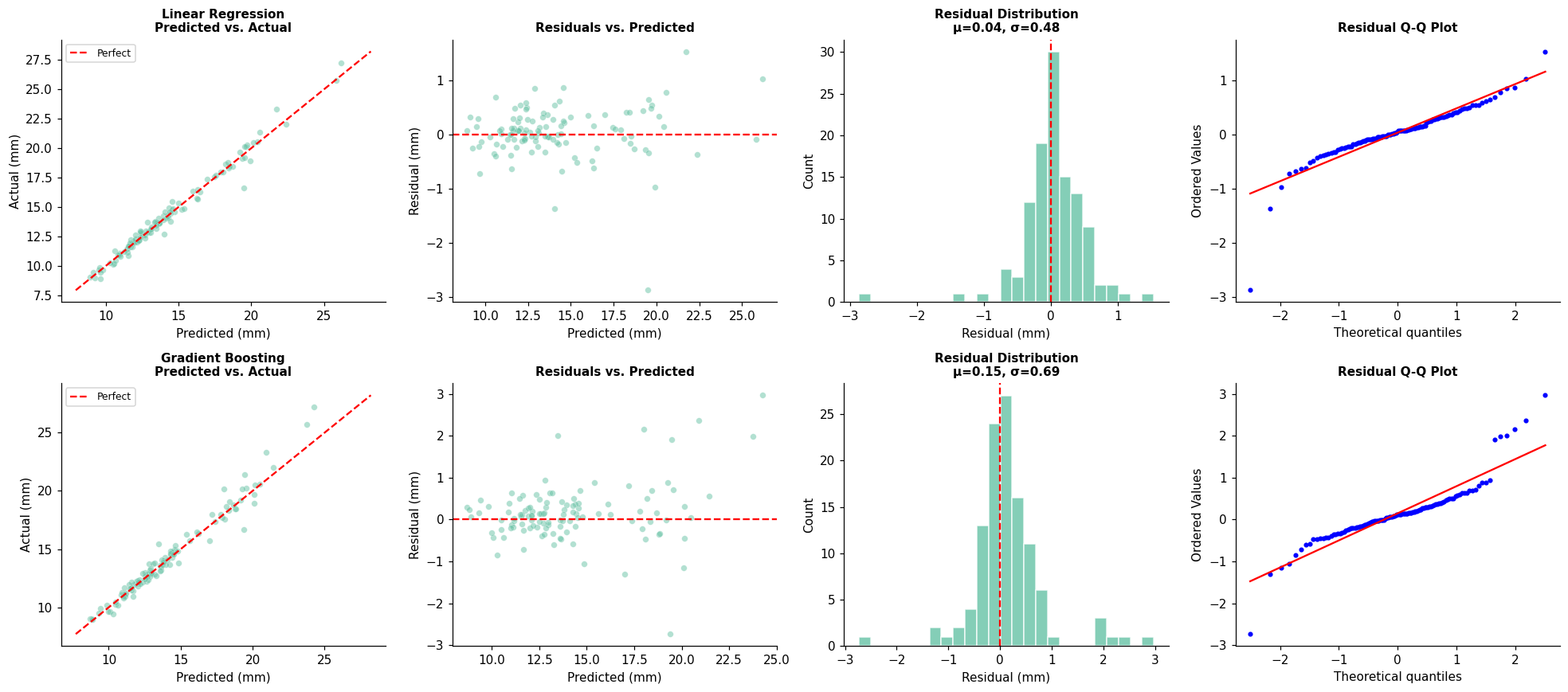
In classification, we checked calibration and discrimination. In regression, the primary diagnostic tool is residual analysis: examining the pattern of errors \(r_i = y_i - \hat{y}_i\) to diagnose model failures.

A well-specified model should have residuals that are:

• Centered around 0 (no systematic bias)

• Roughly constant variance (homoscedasticity)

• Approximately normally distributed

• Independent of the predicted value

from sklearn.linear_model import LinearRegression
from sklearn.ensemble import GradientBoostingRegressor

# ── Train sklearn models ─────────────────────────────────────────────────────
lr_model = LinearRegression()
lr_model.fit(X_train, y_train)

gb_model = GradientBoostingRegressor(n_estimators=200, max_depth=3, learning_rate=0.1,
                                      random_state=42)
gb_model.fit(X_train, y_train)

# Predictions
yhat_lr_val = lr_model.predict(X_val)
yhat_gb_val = gb_model.predict(X_val)

print(f"Linear Regression  — Val MSE: {mse_loss(y_val, yhat_lr_val):.4f}, "
      f"Val MAE: {mae_loss(y_val, yhat_lr_val):.4f}")
print(f"Gradient Boosting  — Val MSE: {mse_loss(y_val, yhat_gb_val):.4f}, "
      f"Val MAE: {mae_loss(y_val, yhat_gb_val):.4f}")

---------------------------------------------------------------------------
NameError                                 Traceback (most recent call last)
Cell In[12], line 16
     12 # Predictions
     13 yhat_lr_val = lr_model.predict(X_val)
     14 yhat_gb_val = gb_model.predict(X_val)
     15 
---> 16 print(f"Linear Regression  — Val MSE: {mse_loss(y_val, yhat_lr_val):.4f}, "
     17       f"Val MAE: {mae_loss(y_val, yhat_lr_val):.4f}")
     18 print(f"Gradient Boosting  — Val MSE: {mse_loss(y_val, yhat_gb_val):.4f}, "
     19       f"Val MAE: {mae_loss(y_val, yhat_gb_val):.4f}")

NameError: name 'mse_loss' is not defined

# ── Residual diagnostic plots ────────────────────────────────────────────────

def residual_diagnostic_panel(y_true, y_pred, model_name, axes_row):
    """Create a row of 4 residual diagnostic plots."""
    residuals = y_true - y_pred

    # 1. Predicted vs. Actual
    ax = axes_row[0]
    ax.scatter(y_pred, y_true, alpha=0.5, s=25, edgecolors='white', linewidth=0.3)
    lims = [min(y_true.min(), y_pred.min()) - 1, max(y_true.max(), y_pred.max()) + 1]
    ax.plot(lims, lims, 'r--', linewidth=1.5, label='Perfect')
    ax.set_xlabel('Predicted (mm)')
    ax.set_ylabel('Actual (mm)')
    ax.set_title(f'{model_name}\nPredicted vs. Actual', fontweight='bold', fontsize=10)
    ax.legend(fontsize=8)

    # 2. Residuals vs. Predicted
    ax = axes_row[1]
    ax.scatter(y_pred, residuals, alpha=0.5, s=25, edgecolors='white', linewidth=0.3)
    ax.axhline(0, color='red', linestyle='--', linewidth=1.5)
    ax.set_xlabel('Predicted (mm)')
    ax.set_ylabel('Residual (mm)')
    ax.set_title('Residuals vs. Predicted', fontweight='bold', fontsize=10)

    # 3. Residual histogram
    ax = axes_row[2]
    ax.hist(residuals, bins=25, color=sns.color_palette('Set2')[0], edgecolor='white', alpha=0.8)
    ax.axvline(0, color='red', linestyle='--', linewidth=1.5)
    ax.set_xlabel('Residual (mm)')
    ax.set_ylabel('Count')
    ax.set_title(f'Residual Distribution\nμ={residuals.mean():.2f}, σ={residuals.std():.2f}',
                 fontweight='bold', fontsize=10)

    # 4. Q-Q plot
    ax = axes_row[3]
    stats.probplot(residuals, dist='norm', plot=ax)
    ax.set_title('Residual Q-Q Plot', fontweight='bold', fontsize=10)
    ax.get_lines()[0].set_markersize(3)


fig, axes = plt.subplots(2, 4, figsize=(18, 8))
residual_diagnostic_panel(y_val, yhat_lr_val, 'Linear Regression', axes[0])
residual_diagnostic_panel(y_val, yhat_gb_val, 'Gradient Boosting', axes[1])
plt.tight_layout()
plt.show()

# ── Test for heteroscedasticity ──────────────────────────────────────────────
# Do residuals "fan out" for larger predicted values?

fig, axes = plt.subplots(1, 2, figsize=(13, 4.5))

for ax, y_pred, name in zip(axes, [yhat_lr_val, yhat_gb_val],
                              ['Linear Regression', 'Gradient Boosting']):
    residuals = y_val - y_pred
    abs_residuals = np.abs(residuals)

    ax.scatter(y_pred, abs_residuals, alpha=0.5, s=25, edgecolors='white', linewidth=0.3)

    # Add a LOESS-like trend line using binned averages
    n_bins = 8
    bins = np.linspace(y_pred.min(), y_pred.max(), n_bins + 1)
    bin_centers, bin_means = [], []
    for j in range(n_bins):
        mask = (y_pred >= bins[j]) & (y_pred < bins[j+1])
        if mask.sum() > 2:
            bin_centers.append((bins[j] + bins[j+1]) / 2)
            bin_means.append(abs_residuals[mask].mean())
    ax.plot(bin_centers, bin_means, 'r-o', linewidth=2, markersize=5, label='Binned mean |residual|')

    ax.set_xlabel('Predicted (mm)')
    ax.set_ylabel('|Residual| (mm)')
    ax.set_title(f'{name}\nHeteroscedasticity Check', fontweight='bold')
    ax.legend(fontsize=9)

plt.tight_layout()
plt.show()

print("If the red trend line slopes upward, residuals grow with predicted value")
print("→ heteroscedasticity: the model's error depends on the prediction magnitude.")
print("This is common in medical measurements: larger tumors are harder to measure precisely.")

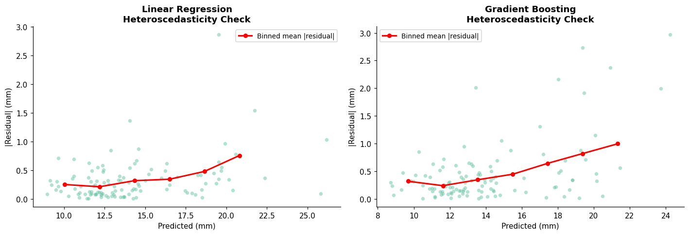
If the red trend line slopes upward, residuals grow with predicted value
→ heteroscedasticity: the model's error depends on the prediction magnitude.
This is common in medical measurements: larger tumors are harder to measure precisely.

🤔 Reflection 4.1 — Residual Patterns

1. In the “Residuals vs. Predicted” plot, do the residuals appear randomly scattered around 0, or do you see a pattern? If there’s a fan-shape (residuals grow with \(\hat{y}\)), what does that tell you about the model’s assumptions?

2. You observe that residuals are larger for bigger tumors. What does this mean clinically? (A model might predict a 10 mm tumor within \(\pm 0.5\) mm but a 25 mm tumor within \(\pm 3\) mm.) Should the loss function account for this? (Foreshadowing: Lab 9 on probabilistic regression will address this directly.)

3. Compare the Linear Regression and Gradient Boosting residual plots. Does the nonlinear model fix any systematic patterns visible in the linear model’s residuals?

---

Part 5 — Evaluation Metrics for Regression

Classification had accuracy, AUROC, F1. Regression has its own family of metrics.

def r_squared_solution(y, y_hat):
    """Coefficient of determination R²."""
    ss_res = np.sum((y - y_hat) ** 2)
    ss_tot = np.sum((y - np.mean(y)) ** 2)
    return 1 - ss_res / ss_tot

# Verify
from sklearn.metrics import r2_score
y_demo = np.array([3, 5, 7, 9, 11.0])
yhat_demo = np.array([3.2, 4.8, 7.1, 8.5, 11.5])
print(f"R² (ours):    {r_squared_solution(y_demo, yhat_demo):.6f}")
print(f"R² (sklearn): {r2_score(y_demo, yhat_demo):.6f}")

# Mean prediction → R² ≈ 0
print(f"R² of mean:   {r_squared_solution(y_demo, np.full_like(y_demo, y_demo.mean())):.6f}")

# Terrible prediction → R² < 0
print(f"R² of 100:    {r_squared_solution(y_demo, np.full_like(y_demo, 100.0)):.2f}")

R² (ours):    0.985250
R² (sklearn): 0.985250
R² of mean:   0.000000
R² of 100:    -1081.12

# ── Comprehensive metrics comparison ─────────────────────────────────────────
from sklearn.metrics import mean_absolute_error, median_absolute_error

def compute_regression_metrics(y_true, y_pred, label=''):
    """Compute and print a full set of regression metrics."""
    mse_val  = mse_loss(y_true, y_pred)
    rmse_val = np.sqrt(mse_val)
    mae_val  = mae_loss(y_true, y_pred)
    med_ae   = median_absolute_error(y_true, y_pred)
    r2_val   = r_squared(y_true, y_pred)

    return {
        'Model': label,
        'MSE (mm²)': mse_val,
        'RMSE (mm)': rmse_val,
        'MAE (mm)': mae_val,
        'MedAE (mm)': med_ae,
        'R²': r2_val
    }


metrics = [
    compute_regression_metrics(y_val, yhat_lr_val, 'Linear Regression'),
    compute_regression_metrics(y_val, yhat_gb_val, 'Gradient Boosting'),
    compute_regression_metrics(y_val, np.full_like(y_val, y_train.mean()), 'Predict Mean (baseline)'),
]

metrics_df = pd.DataFrame(metrics).set_index('Model')
print(metrics_df.to_string(float_format='%.4f'))

print("\n" + "─" * 70)
print("Metric guide:")
print("  MSE:   Mean Squared Error — in mm², penalizes large errors heavily")
print("  RMSE:  Root MSE — in mm, same units as target")
print("  MAE:   Mean Absolute Error — in mm, robust to outliers")
print("  MedAE: Median Absolute Error — in mm, even more robust")
print("  R²:    1 = perfect, 0 = no better than mean, <0 = worse than mean")

---------------------------------------------------------------------------
NameError                                 Traceback (most recent call last)
Cell In[16], line 23
     19     }
     20 
     21 
     22 metrics = [
---> 23     compute_regression_metrics(y_val, yhat_lr_val, 'Linear Regression'),
     24     compute_regression_metrics(y_val, yhat_gb_val, 'Gradient Boosting'),
     25     compute_regression_metrics(y_val, np.full_like(y_val, y_train.mean()), 'Predict Mean (baseline)'),
     26 ]

Cell In[16], line 6, in compute_regression_metrics(y_true, y_pred, label)
      4 def compute_regression_metrics(y_true, y_pred, label=''):
      5     """Compute and print a full set of regression metrics."""
----> 6     mse_val  = mse_loss(y_true, y_pred)
      7     rmse_val = np.sqrt(mse_val)
      8     mae_val  = mae_loss(y_true, y_pred)
      9     med_ae   = median_absolute_error(y_true, y_pred)

NameError: name 'mse_loss' is not defined

🤔 Reflection 5.1 — Interpreting Regression Metrics

1. Can \(R^2\) be negative? What does it mean when a model achieves \(R^2 < 0\)? Under what circumstances might this happen in practice?

2. A model achieves \(R^2 = 0.95\) on your test set. Does that mean it’s clinically useful? What additional information would you need? (Hint: \(R^2 = 0.95\) with an RMSE of 3 mm might be fine for treatment planning but terrible for a micro-surgical measurement.)

3. RMSE and MAE are in the same units (mm) but often differ. When RMSE \(\gg\) MAE, what does that imply? (Hint: RMSE is more sensitive to large errors, so a big gap means there are some samples with very large errors — outliers or hard cases.)

---

Part 6 — Log-Transformed Targets

When the target is positive and right-skewed (as tumor radius is), applying a log-transform before fitting can improve model performance. This is because:

• Log-transform reduces skewness, making the distribution more Gaussian-like

• MSE in log-space penalizes relative errors rather than absolute errors: \(\log(\hat{y}) - \log(y) = \log(\hat{y}/y)\)

• This often matches clinical intuition: a 1 mm error on a 5 mm tumor is more concerning than a 1 mm error on a 25 mm tumor

# ── Log-transform the target ─────────────────────────────────────────────────
y_train_log = np.log(y_train)
y_val_log   = np.log(y_val)
y_test_log  = np.log(y_test)

fig, axes = plt.subplots(1, 2, figsize=(12, 4))

axes[0].hist(y_train, bins=30, color=sns.color_palette('Set2')[0], edgecolor='white', alpha=0.8)
axes[0].set_xlabel('Mean Radius (mm)')
axes[0].set_ylabel('Count')
axes[0].set_title(f'Original Scale\nSkewness={stats.skew(y_train):.3f}', fontweight='bold')

axes[1].hist(y_train_log, bins=30, color=sns.color_palette('Set2')[2], edgecolor='white', alpha=0.8)
axes[1].set_xlabel('log(Mean Radius)')
axes[1].set_ylabel('Count')
axes[1].set_title(f'Log-Transformed\nSkewness={stats.skew(y_train_log):.3f}', fontweight='bold')

plt.tight_layout()
plt.show()

print(f"Skewness reduced: {stats.skew(y_train):.3f} → {stats.skew(y_train_log):.3f}")

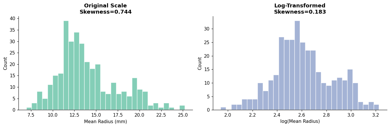
Skewness reduced: 0.744 → 0.183

# ── Train models in log-space ────────────────────────────────────────────────
lr_log = LinearRegression()
lr_log.fit(X_train, y_train_log)

gb_log = GradientBoostingRegressor(n_estimators=200, max_depth=3, learning_rate=0.1,
                                    random_state=42)
gb_log.fit(X_train, y_train_log)

# Predictions in log-space → transform back to original
yhat_lr_log_val = np.exp(lr_log.predict(X_val))
yhat_gb_log_val = np.exp(gb_log.predict(X_val))

# Compare metrics in ORIGINAL space (mm)
print("Metrics in original mm scale:")
print("─" * 70)

models_compare = [
    ('Linear (orig. scale)',  yhat_lr_val),
    ('Linear (log → exp)',    yhat_lr_log_val),
    ('GBR (orig. scale)',     yhat_gb_val),
    ('GBR (log → exp)',       yhat_gb_log_val),
]

rows = []
for name, yhat in models_compare:
    rows.append(compute_regression_metrics(y_val, yhat, name))

compare_df = pd.DataFrame(rows).set_index('Model')
print(compare_df.to_string(float_format='%.4f'))

Metrics in original mm scale:
──────────────────────────────────────────────────────────────────────

---------------------------------------------------------------------------
NameError                                 Traceback (most recent call last)
Cell In[18], line 26
     22 ]
     23 
     24 rows = []
     25 for name, yhat in models_compare:
---> 26     rows.append(compute_regression_metrics(y_val, yhat, name))
     27 
     28 compare_df = pd.DataFrame(rows).set_index('Model')
     29 print(compare_df.to_string(float_format='%.4f'))

Cell In[16], line 6, in compute_regression_metrics(y_true, y_pred, label)
      4 def compute_regression_metrics(y_true, y_pred, label=''):
      5     """Compute and print a full set of regression metrics."""
----> 6     mse_val  = mse_loss(y_true, y_pred)
      7     rmse_val = np.sqrt(mse_val)
      8     mae_val  = mae_loss(y_true, y_pred)
      9     med_ae   = median_absolute_error(y_true, y_pred)

NameError: name 'mse_loss' is not defined

# ── Compare residual patterns: original vs. log-transformed ──────────────────
fig, axes = plt.subplots(1, 2, figsize=(13, 4.5))

# Linear: original scale residuals
res_orig = y_val - yhat_lr_val
axes[0].scatter(yhat_lr_val, res_orig, alpha=0.5, s=25, edgecolors='white', linewidth=0.3)
axes[0].axhline(0, color='red', linestyle='--', linewidth=1.5)
axes[0].set_xlabel('Predicted (mm)')
axes[0].set_ylabel('Residual (mm)')
axes[0].set_title('Linear Regression (original scale)', fontweight='bold')

# Linear: log-transformed residuals
res_log = y_val - yhat_lr_log_val
axes[1].scatter(yhat_lr_log_val, res_log, alpha=0.5, s=25, edgecolors='white', linewidth=0.3)
axes[1].axhline(0, color='red', linestyle='--', linewidth=1.5)
axes[1].set_xlabel('Predicted (mm)')
axes[1].set_ylabel('Residual (mm)')
axes[1].set_title('Linear Regression (log-transformed)', fontweight='bold')

plt.tight_layout()
plt.show()

print("Does the log-transform reduce the heteroscedasticity (fanning pattern)?")
print("MSE in log-space ≈ penalizing relative errors, which often makes residuals more uniform.")

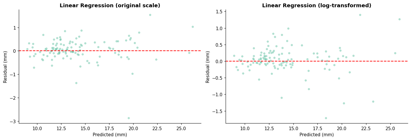
Does the log-transform reduce the heteroscedasticity (fanning pattern)?
MSE in log-space ≈ penalizing relative errors, which often makes residuals more uniform.

🤔 Reflection 6.1 — When to Transform the Target

1. When is it appropriate to apply a log-transform to the target? What assumptions does it encode? (Hint: it assumes multiplicative noise rather than additive.)

2. MSE in log-space corresponds to minimizing \(\frac{1}{n} \sum (\log \hat{y}_i - \log y_i)^2 = \frac{1}{n} \sum \left(\log \frac{\hat{y}_i}{y_i}\right)^2\). This penalizes relative errors equally: over-predicting by 2× is penalized the same as under-predicting by 2×, regardless of the absolute tumor size. When is this more appropriate than penalizing absolute mm errors?

3. After back-transforming (\(\hat{y} = \exp(\hat{y}_{\log})\)), the predictions approximate the conditional geometric mean rather than the arithmetic mean. For right-skewed distributions, the geometric mean < arithmetic mean. Does this matter clinically?

---

Part 7 — Final Test Set Evaluation

Following the same protocol as all previous labs: evaluate on the test set once, using the model and configuration chosen on the validation set.

# ── Final test set evaluation ────────────────────────────────────────────────
# Use Gradient Boosting (original scale) as the best model based on val metrics

# Retrain on train + val
X_tv  = np.vstack([X_train, X_val])
y_tv  = np.concatenate([y_train, y_val])

final_gb = GradientBoostingRegressor(n_estimators=200, max_depth=3, learning_rate=0.1,
                                      random_state=42)
final_gb.fit(X_tv, y_tv)

yhat_test_final = final_gb.predict(X_test)

print("═" * 65)
print("  FINAL TEST SET EVALUATION — Gradient Boosting Regressor")
print("═" * 65)

final_metrics = compute_regression_metrics(y_test, yhat_test_final, 'Final GBR')
for k, v in final_metrics.items():
    if k != 'Model':
        print(f"  {k:12s}: {v:.4f}")
print("═" * 65)

═════════════════════════════════════════════════════════════════
  FINAL TEST SET EVALUATION — Gradient Boosting Regressor
═════════════════════════════════════════════════════════════════

---------------------------------------------------------------------------
NameError                                 Traceback (most recent call last)
Cell In[20], line 18
     14 print("═" * 65)
     15 print("  FINAL TEST SET EVALUATION — Gradient Boosting Regressor")
     16 print("═" * 65)
     17 
---> 18 final_metrics = compute_regression_metrics(y_test, yhat_test_final, 'Final GBR')
     19 for k, v in final_metrics.items():
     20     if k != 'Model':
     21         print(f"  {k:12s}: {v:.4f}")

Cell In[16], line 6, in compute_regression_metrics(y_true, y_pred, label)
      4 def compute_regression_metrics(y_true, y_pred, label=''):
      5     """Compute and print a full set of regression metrics."""
----> 6     mse_val  = mse_loss(y_true, y_pred)
      7     rmse_val = np.sqrt(mse_val)
      8     mae_val  = mae_loss(y_true, y_pred)
      9     med_ae   = median_absolute_error(y_true, y_pred)

NameError: name 'mse_loss' is not defined

# ── Test set diagnostic plots ────────────────────────────────────────────────
fig, axes = plt.subplots(1, 3, figsize=(15, 4.5))

residuals_test = y_test - yhat_test_final

# Predicted vs. Actual
axes[0].scatter(yhat_test_final, y_test, alpha=0.5, s=30, edgecolors='white', linewidth=0.3)
lims = [min(y_test.min(), yhat_test_final.min()) - 1,
        max(y_test.max(), yhat_test_final.max()) + 1]
axes[0].plot(lims, lims, 'r--', linewidth=1.5, label='Perfect')
axes[0].set_xlabel('Predicted (mm)')
axes[0].set_ylabel('Actual (mm)')
axes[0].set_title('Predicted vs. Actual (Test)', fontweight='bold')
axes[0].legend()

# Residuals vs. Predicted
axes[1].scatter(yhat_test_final, residuals_test, alpha=0.5, s=30, edgecolors='white', linewidth=0.3)
axes[1].axhline(0, color='red', linestyle='--', linewidth=1.5)
axes[1].set_xlabel('Predicted (mm)')
axes[1].set_ylabel('Residual (mm)')
axes[1].set_title('Residuals vs. Predicted (Test)', fontweight='bold')

# Error distribution
axes[2].hist(residuals_test, bins=25, color=sns.color_palette('Set2')[0], edgecolor='white', alpha=0.8)
axes[2].axvline(0, color='red', linestyle='--', linewidth=1.5)
axes[2].set_xlabel('Residual (mm)')
axes[2].set_ylabel('Count')
axes[2].set_title(f'Test Residuals\nRMSE={np.sqrt(mse_loss(y_test, yhat_test_final)):.2f} mm',
                   fontweight='bold')

plt.tight_layout()
plt.show()

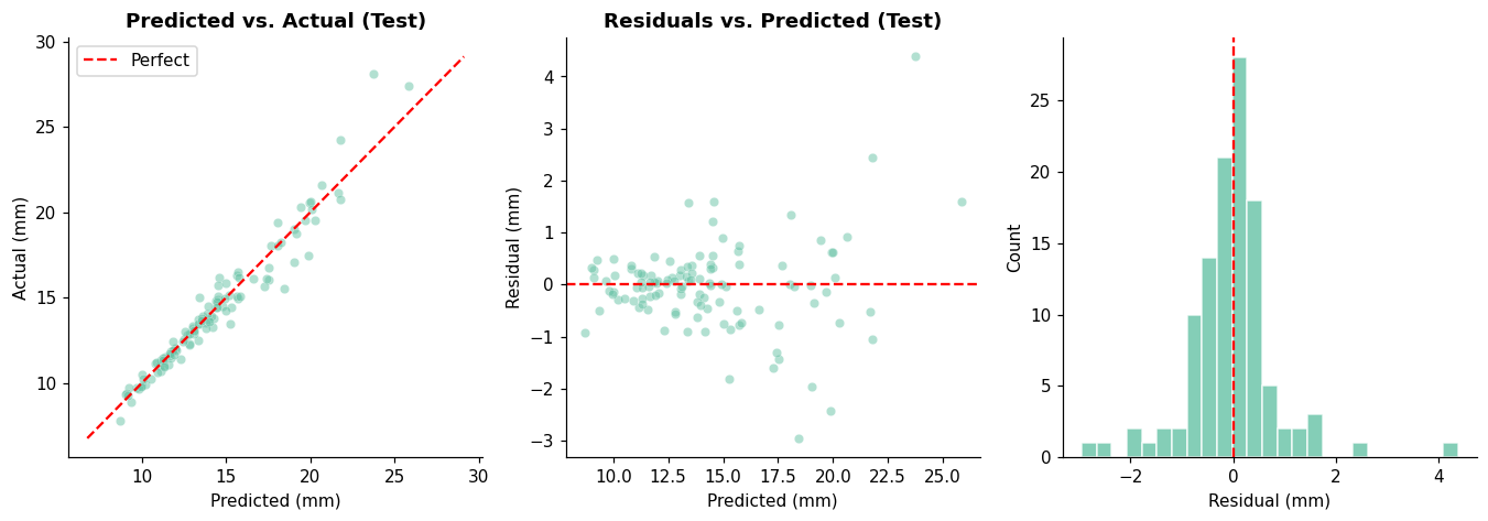
print(f"\nThe model predicts tumor radius with RMSE ≈ {np.sqrt(mse_loss(y_test, yhat_test_final)):.2f} mm")
print(f"and MAE ≈ {mae_loss(y_test, yhat_test_final):.2f} mm on held-out patients.")

---------------------------------------------------------------------------
NameError                                 Traceback (most recent call last)
Cell In[21], line 28
     24 axes[2].hist(residuals_test, bins=25, color=sns.color_palette('Set2')[0], edgecolor='white', alpha=0.8)
     25 axes[2].axvline(0, color='red', linestyle='--', linewidth=1.5)
     26 axes[2].set_xlabel('Residual (mm)')
     27 axes[2].set_ylabel('Count')
---> 28 axes[2].set_title(f'Test Residuals\nRMSE={np.sqrt(mse_loss(y_test, yhat_test_final)):.2f} mm',
     29                    fontweight='bold')
     30 
     31 plt.tight_layout()

NameError: name 'mse_loss' is not defined

---

🤔 Final Reflection

You’re building a model to predict hospital length-of-stay (LOS) — a positive, right-skewed continuous variable where most patients stay 1–3 days but some stay weeks.

1. Loss function: Which loss would you start with — MSE, MAE, or Huber — and why? Would you log-transform the target? What clinical considerations influence this choice? (Hint: a 1-day error for a patient staying 2 days is very different from a 1-day error for a patient staying 30 days.)

2. Outliers and data quality: Hospital LOS data often has coding errors (e.g., patients recorded as staying 365 days due to administrative issues). How would each loss function handle these? Which is most dangerous to leave uncorrected?

3. Clinical utility beyond \(R^2\): An \(R^2\) of 0.70 sounds decent, but how would you communicate model performance to a hospital administrator? They want to know: “Can I trust this model to plan bed allocation?” What metrics and visualizations would you show them? (Consider: RMSE in interpretable units, prediction intervals, calibration plots of predicted vs. actual LOS.)

4. Connection to Lab 9: This lab produced point estimates — a single predicted value per patient. But the residual analysis showed that prediction uncertainty varies by patient (heteroscedasticity). Lab 9 will address this by predicting distributions instead of points. How might that change your answer to question 3?