
🌲 Lab 2: Decision Trees#
BINF 4002 – Machine Learning for Health
Learning Objectives#
Understand how decision trees partition feature space using information-theoretic criteria
Build, visualize, and manually trace a decision tree
Implement tree prediction yourself and validate it
Demonstrate and explain overfitting in trees
Understand regularization strategies for trees
What is a Decision Tree?#
A decision tree is a model that makes predictions by recursively partitioning the input space into rectangular regions, one split at a time. At each internal node, the algorithm asks: which feature, and which threshold on that feature, best separates the classes in my current subset of training data? The best split is chosen by maximizing information gain — the reduction in impurity achieved by making the split.
The most common impurity measure for classification is the Gini impurity:
where \(p_k\) is the fraction of samples in set \(S\) belonging to class \(k\). A pure node (all one class) has \(G=0\); a maximally mixed node has \(G=0.5\) for binary classification. The algorithm greedily picks the split that minimizes the weighted average Gini of the two child nodes:
where \(S_L, S_R\) are the subsets falling left and right of threshold \(t\) on feature \(j\).
This process repeats recursively in each child node until a stopping criterion is met (maximum depth, minimum samples per leaf, or no further gain). Prediction is then simply: trace the sample from root to a leaf, and return the majority class in that leaf.
Why do we care about decision trees in healthcare? Three reasons. First, the prediction rule is completely explicit — you can print it out and hand it to a clinician. Second, trees naturally handle mixed feature types (continuous, ordinal) without requiring scaling. Third, and most importantly for this course, understanding trees is the prerequisite for understanding random forests and gradient boosting, which are among the best-performing models on structured clinical data.
Set-up#
Upload data#
⚠️ First, you need to upload the pre-processed data from lab0. If you have issues with running the first lab, you can also download the data here.
Once you have downloaded the data locally and started the runtime for this notebook, upload the file via the “Files” menu.
import os, pickle, warnings
import numpy as np
import pandas as pd
import matplotlib.pyplot as plt
import seaborn as sns
warnings.filterwarnings('ignore')

plt.rcParams['figure.dpi'] = 110
plt.rcParams['axes.spines.top'] = False
plt.rcParams['axes.spines.right'] = False

pkl_path = 'processed_data.pkl'
if not os.path.exists(pkl_path):
    raise FileNotFoundError(
        "processed_data.pkl not found. Run Lab 0 first, or download the data "
        "from the link above and upload it here."
    )

with open(pkl_path, 'rb') as f:
    d = pickle.load(f)

# Use the *restricted* hard splits (8 weakest features, 120 train samples)
# This gives realistic AUC rather than a trivially easy problem.
X_train, y_train = d['X_train_hard'], d['y_train_hard']
X_val,   y_val   = d['X_val_hard'],   d['y_val_hard']
X_test,  y_test  = d['X_test_hard'],  d['y_test_hard']
feature_names    = d['feature_names_hard']
class_names      = ['Malignant', 'Benign']

print(f"Train : {X_train.shape}  |  Val : {X_val.shape}  |  Test : {X_test.shape}")
print(f"Features: {feature_names}")
Train : (100, 8)  |  Val : (114, 8)  |  Test : (114, 8)
Features: ['mean symmetry', 'compactness error', 'concavity error', 'smoothness error', 'texture error', 'fractal dimension error', 'symmetry error', 'mean fractal dimension']
from sklearn.metrics import confusion_matrix, roc_auc_score

def print_metrics(y_true, y_pred, y_prob=None, label='Model'):
    tn,fp,fn,tp = confusion_matrix(y_true, y_pred).ravel()
    n = len(y_true)
    sens = tp/(tp+fn); spec = tn/(tn+fp)
    ppv  = tp/(tp+fp); npv  = tn/(tn+fn)
    prev = (tp+fn)/n
    print(f"{'─'*55}")
    print(f"  {label}")
    print(f"{'─'*55}")
    print(f"  Sensitivity  P(ŷ=1|y=1)  = {tp}/{tp+fn} = {sens:.3f}")
    print(f"  Specificity  P(ŷ=0|y=0)  = {tn}/{tn+fp} = {spec:.3f}")
    print(f"  PPV          P(y=1|ŷ=1)  = {tp}/{tp+fp} = {ppv:.3f}")
    print(f"  NPV          P(y=0|ŷ=0)  = {tn}/{tn+fn} = {npv:.3f}")
    print(f"  Prevalence               = {prev:.3f}")
    if y_prob is not None:
        auc = roc_auc_score(y_true, y_prob)
        print(f"  AUC-ROC                  = {auc:.3f}")
    print()
Part 1 — Build and Visualize a Decision Tree#
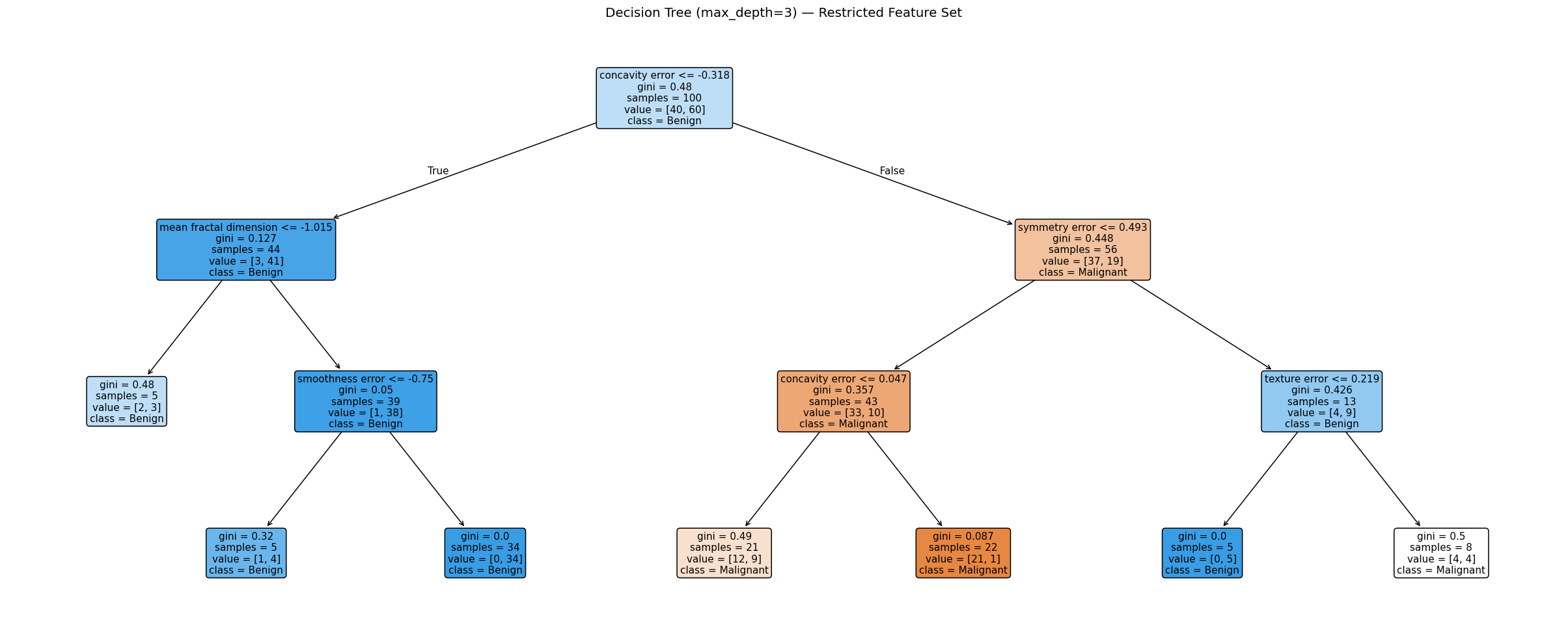
We start with a shallow tree (max_depth=3) so the full structure is visible. Before running
the cell, make a prediction: given only 8 weakly-informative features and 120 training
samples, how well do you think this tree will do on the validation set?
from sklearn.tree import DecisionTreeClassifier, plot_tree, export_text

dt3 = DecisionTreeClassifier(max_depth=3, min_samples_leaf=5, random_state=42)
dt3.fit(X_train, y_train)

plt.figure(figsize=(22, 9))
plot_tree(dt3,
          feature_names=feature_names,
          class_names=class_names,
          filled=True, rounded=True, fontsize=10,
          impurity=True, proportion=False)
plt.title('Decision Tree (max_depth=3) — Restricted Feature Set', fontsize=13)
plt.tight_layout(); plt.show()

print("\nText representation:")
print(export_text(dt3, feature_names=feature_names))

val_preds = dt3.predict(X_val)
val_probs = dt3.predict_proba(X_val)[:, 1]
print_metrics(y_val, val_preds, val_probs, label='Decision Tree (depth=3), Validation')
Text representation:
|--- concavity error <= -0.32
|   |--- mean fractal dimension <= -1.02
|   |   |--- class: 1
|   |--- mean fractal dimension >  -1.02
|   |   |--- smoothness error <= -0.75
|   |   |   |--- class: 1
|   |   |--- smoothness error >  -0.75
|   |   |   |--- class: 1
|--- concavity error >  -0.32
|   |--- symmetry error <= 0.49
|   |   |--- concavity error <= 0.05
|   |   |   |--- class: 0
|   |   |--- concavity error >  0.05
|   |   |   |--- class: 0
|   |--- symmetry error >  0.49
|   |   |--- texture error <= 0.22
|   |   |   |--- class: 1
|   |   |--- texture error >  0.22
|   |   |   |--- class: 0

───────────────────────────────────────────────────────
  Decision Tree (depth=3), Validation
───────────────────────────────────────────────────────
  Sensitivity  P(ŷ=1|y=1)  = 49/72 = 0.681
  Specificity  P(ŷ=0|y=0)  = 36/42 = 0.857
  PPV          P(y=1|ŷ=1)  = 49/55 = 0.891
  NPV          P(y=0|ŷ=0)  = 36/59 = 0.610
  Prevalence               = 0.632
  AUC-ROC                  = 0.795
Understanding the Tree Output#
Each node in the visualization shows:
The split condition (e.g.,
mean texture ≤ 0.32)Gini impurity of the node — 0.0 is pure, 0.5 is maximally mixed
samples — how many training examples reach this node
value — the count of [malignant, benign] examples at this node
class — the majority class (what would be predicted if we stopped here)
The color intensity reflects purity: darker = more confident. Notice how Gini impurity decreases as you move from root to leaves — this is the information gain the algorithm is maximizing at each step.
🤔 Reflection 1.1 — Reading the Tree#
Look at the root node’s Gini impurity and the Gini impurities of its two children. Compute the information gain of the first split by hand. Does this match what sklearn would compute?
Find a leaf node with high Gini impurity (close to 0.5). What does this mean clinically? Would you trust a model that routes many patients to this leaf?
The tree splits only on continuous thresholds. If a feature were ordinal (e.g., tumor grade 1–4), how would the tree handle it? What assumption does this implicitly make about the ordering?
✅ Solution — Reflection 1.1#
1. Information gain of the root split: The root node has some Gini impurity \(G_{\text{root}}\). After splitting, the two children have impurities \(G_L\) and \(G_R\) with sizes \(n_L\) and \(n_R\). Information gain = \(G_{\text{root}} - \frac{n_L}{n}G_L - \frac{n_R}{n}G_R\). You can verify this by reading the Gini, sample counts, and class distributions from the tree visualization. For example, if the root has Gini=0.48 with 100 samples, and splits into a left child with Gini=0.127 (44 samples) and right child with Gini=0.448 (56 samples), the gain = 0.48 − (44/100)(0.127) − (56/100)(0.448) = 0.1732.
2. A leaf node with high Gini (close to 0.5) means the samples reaching that leaf are nearly evenly split between malignant and benign. The model is uncertain for patients routed there. Clinically, you should not trust a prediction from a high-impurity leaf — it’s essentially a coin flip. These leaves represent regions of feature space where the model lacks discriminative information.
3. For ordinal features like tumor grade (1–4), the tree still splits on thresholds (e.g., “grade ≤ 2”). This implicitly assumes that the classes form contiguous groups along the ordinal scale (e.g., grades 1–2 vs. 3–4). It cannot split on {1, 3} vs. {2, 4} without multiple splits. This assumption is often reasonable for ordinal variables but may miss non-monotonic patterns.
Part 2 — Implement Tree Prediction Yourself#
A decision tree’s prediction is a series of comparisons. Implement a function that traces
a single sample through the tree using sklearn’s internal tree_ object. This exercise
makes explicit that the “model” is just a lookup table of thresholds, and prediction is
just a traversal — O(depth) operations, no matrix multiplication anywhere.
Useful attributes of dt3.tree_:
.feature[node]— which feature is split on at this node (-2 = leaf).threshold[node]— the threshold value for the split.children_left[node]/.children_right[node]— child node indices.value[node]— shape(1, n_classes)array of class counts at this node
# ── SOLUTION ──────────────────────────────────────────────────────────────────
# Implement manual tree traversal for a single sample.

def predict_one_sample_tree(tree_clf, x_sample):
    """
    Manually traverse a fitted DecisionTreeClassifier for a single sample.
    Returns: (predicted_class, list_of_decision_strings)
    """
    tree = tree_clf.tree_
    node = 0       # start at root
    decisions = []

    while tree.feature[node] != -2:   # -2 means leaf
        feat_idx   = tree.feature[node]
        threshold  = tree.threshold[node]
        feat_name  = feature_names[feat_idx]
        feat_value = x_sample[feat_idx]

        if feat_value <= threshold:
            decisions.append(f"{feat_name} = {feat_value:.4f} <= {threshold:.4f} → go LEFT")
            node = tree.children_left[node]
        else:
            decisions.append(f"{feat_name} = {feat_value:.4f} > {threshold:.4f} → go RIGHT")
            node = tree.children_right[node]

    # At a leaf — majority class
    class_counts = tree.value[node][0]
    predicted_class = int(np.argmax(class_counts))
    return predicted_class, decisions


# Test on a validation sample
sample_idx = 3
pred_class, path = predict_one_sample_tree(dt3, X_val[sample_idx])
print(f"Sample {sample_idx}: True label = {class_names[y_val[sample_idx]]}")
print(f"Manual prediction  : {class_names[pred_class]}")
print(f"Sklearn prediction : {class_names[dt3.predict(X_val[[sample_idx]])[0]]}")
print("\nDecision path:")
for step in path:
    print(f"  {step}")
Sample 3: True label = Malignant
Manual prediction  : Malignant
Sklearn prediction : Malignant

Decision path:
  concavity error = 0.2833 > -0.3176 → go RIGHT
  symmetry error = 0.6563 > 0.4934 → go RIGHT
  texture error = 0.5878 > 0.2188 → go RIGHT
# ── Sanity check ──────────────────────────────────────────────────────────────
# Run on all validation samples and compare to sklearn
manual_preds = np.array([predict_one_sample_tree(dt3, x)[0] for x in X_val])
sklearn_preds = dt3.predict(X_val)

n_agree = (manual_preds == sklearn_preds).sum()
assert n_agree == len(X_val), (
    f"Manual predictions disagree with sklearn on {len(X_val)-n_agree} samples. "
    "Check your left/right child logic and the leaf condition."
)
print(f"✓ Manual traversal matches sklearn on all {len(X_val)} validation samples.")
✓ Manual traversal matches sklearn on all 114 validation samples.
🤔 Reflection 2.1 — Trees as Explicit Rules#
Your implementation is a while loop with a handful of comparisons. Compare this to logistic regression’s forward pass (a dot product + sigmoid). Which is more computationally expensive per sample? Which is easier for a non-technical clinician to audit?
You ran the tree manually on a single sample. Could you do this for 200 trees?
How “explainable” is a decision tree? What does “explainability” or “interpretability” mean for this kind of model?
Decision trees split on thresholds of continuous features. This means the decision boundary is always axis-aligned (perpendicular to a feature axis). Draw a 2D example where this makes trees fundamentally not as appropriate logistic regression. Then draw one where trees are more appropriate. Which is more expressive: A decision tree or a logisitic regression model?
✅ Solution — Reflection 2.1#
1. Tree prediction is \(O(\text{depth})\) — a few comparisons per sample (typically 3–10). Logistic regression is \(O(d)\) — a dot product over all features. For small trees and moderate \(d\), tree prediction is actually slightly cheaper. For a clinician, the tree is far easier to audit: “if smoothness > 0.1 and texture ≤ 0.3, predict malignant” is a rule anyone can verify.
2. You could not do this manually for 200 trees. This is the fundamental trade-off with ensemble methods (like Random Forests): they aggregate many trees for better performance, but the ensemble becomes opaque. A single tree is interpretable; 200 trees is a black box (though tools like SHAP can help).
3. A decision tree is “explainable” in a specific sense: for any prediction, you can trace the exact sequence of feature comparisons that led to it, and each comparison has a clear clinical meaning (“was mean texture above or below 0.3?”). This is local interpretability — you can explain why a specific patient got a specific prediction. It also has global interpretability — you can print the entire tree and see all possible decision paths. However, “interpretable” does not mean “correct” or “trustworthy” — an overfit tree gives clear explanations for wrong predictions.
4. Axis-aligned boundaries make trees less appropriate when the true decision boundary is diagonal (e.g., “malignant if radius + 0.5 × texture > 20” — a linear boundary at 45°). The tree would need many staircase-like splits to approximate this. Trees are more appropriate when the decision boundary is rectangular (e.g., “malignant if radius > 15 OR texture > 25” — two perpendicular cuts). Overall, a logistic regression model is more expressive for linear boundaries, while a sufficiently deep tree can approximate any boundary (including linear ones), but may need many more splits to do so. Neither is strictly more expressive — a deep enough tree can represent any partition of the space, but so can logistic regression with feature engineering.
Part 3 — Overfitting: A Practical Demonstration#
Decision trees can memorize training data perfectly — a critical failure mode in clinical settings where we need the model to generalize to new patients, not recall training cases. With only 120 training examples and 8 features, overfitting happens very quickly.
Before running: at what depth do you expect the training accuracy to reach 100%? At what depth do you expect validation accuracy to peak?
depths = list(range(1, 25))
train_accs, val_accs, train_aucs, val_aucs = [], [], [], []

for depth in depths:
    dt = DecisionTreeClassifier(max_depth=depth, random_state=42)
    dt.fit(X_train, y_train)
    train_accs.append(dt.score(X_train, y_train))
    val_accs.append(dt.score(X_val, y_val))
    train_aucs.append(roc_auc_score(y_train, dt.predict_proba(X_train)[:,1]))
    val_aucs.append(roc_auc_score(y_val,   dt.predict_proba(X_val)[:,1]))

best_depth = depths[np.argmax(val_accs)]

fig, axes = plt.subplots(1, 2, figsize=(14, 5))

for ax, metric, train_vals, val_vals, ylabel in zip(
    axes,
    ['Accuracy', 'AUC-ROC'],
    [train_accs, train_aucs],
    [val_accs, val_aucs],
    ['Accuracy', 'AUC-ROC']
):
    ax.plot(depths, train_vals, 'o-', color='#3498db', lw=2, label='Train')
    ax.plot(depths, val_vals,   's-', color='#e74c3c', lw=2, label='Val')
    ax.axvline(best_depth, color='grey', linestyle='--', alpha=0.7,
               label=f'Best depth = {best_depth}')
    ax.set_xlabel('Max depth'); ax.set_ylabel(ylabel)
    ax.set_title(f'{ylabel} vs. Tree Depth (n_train=120)')
    ax.legend(); ax.grid(True, alpha=0.3)

plt.tight_layout(); plt.show()

print(f"Best depth (by val accuracy): {best_depth}")
print(f"Train accuracy at depth {best_depth}: {train_accs[best_depth-1]:.3f}")
print(f"Val   accuracy at depth {best_depth}: {val_accs[best_depth-1]:.3f}")
print(f"Train accuracy at depth 20       : {train_accs[19]:.3f}")
print(f"Val   accuracy at depth 20       : {val_accs[19]:.3f}")
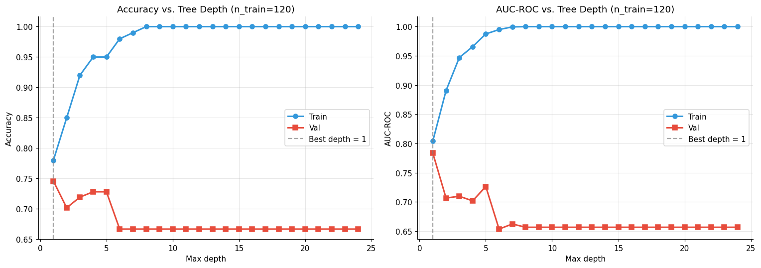
Best depth (by val accuracy): 1
Train accuracy at depth 1: 0.780
Val   accuracy at depth 1: 0.746
Train accuracy at depth 20       : 1.000
Val   accuracy at depth 20       : 0.667
Why Does a Deep Tree Overfit?#
A tree with no depth limit will keep splitting until every leaf contains exactly one training sample, achieving 100% training accuracy but generalizing no better than a lookup table. The fundamental quantity is the number of leaves, which upper-bounds the number of training samples a tree can perfectly classify: a tree with \(L\) leaves can perfectly fit any dataset with \(L\) distinct samples.
For \(n\) training samples, a complete binary tree reaches this at depth \(\lceil \log_2 n \rceil\) — for \(n=120\), that’s depth 7. This gives us a concrete, calibrated intuition: trees deeper than about \(\log_2(n)\) are almost always overfitting.
Given our discussion about memorization vs. interpolation, what might you suspect about ways we could make a decision tree less likely to overfit?
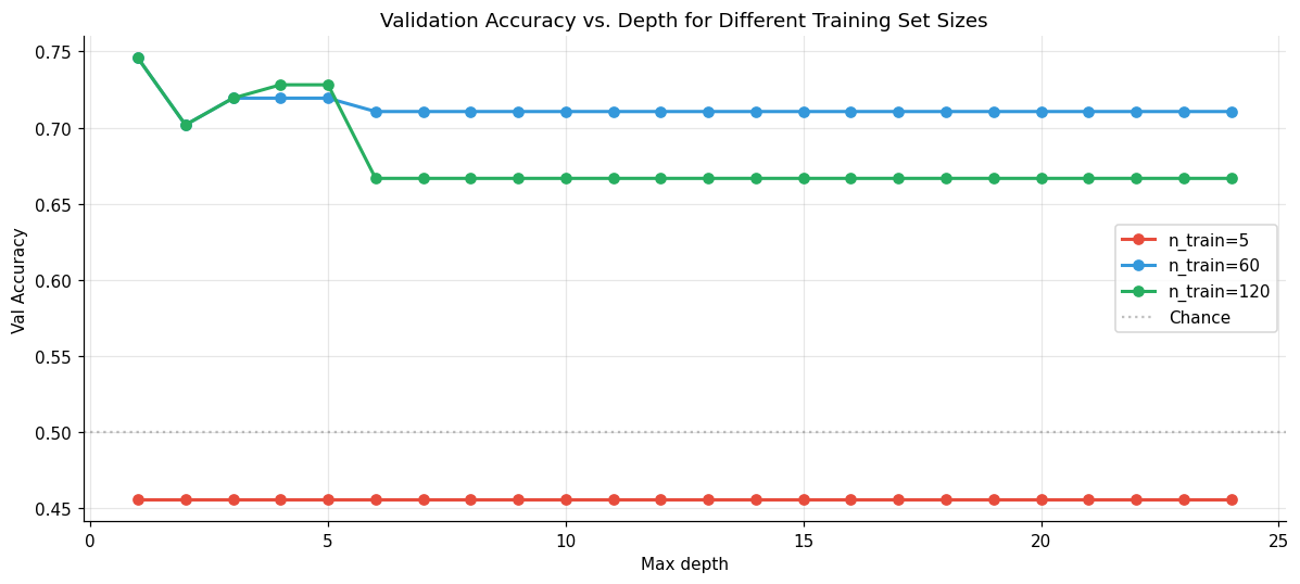
# How does training set size affect the overfitting depth?
# Vary n_train and see at what depth overfitting begins.

fig, ax = plt.subplots(figsize=(11, 5))

for n_train, color in [(5, '#e74c3c'), (60, '#3498db'), (120, '#27ae60')]:
    idx = np.random.RandomState(42).choice(len(X_train), min(n_train, len(X_train)), replace=False)
    Xt, yt = X_train[idx], y_train[idx]
    v_accs = []
    for depth in depths:
        dt = DecisionTreeClassifier(max_depth=depth, random_state=42)
        dt.fit(Xt, yt)
        v_accs.append(dt.score(X_val, y_val))
    ax.plot(depths, v_accs, 'o-', lw=2, label=f'n_train={n_train}', color=color)

ax.axhline(0.5, color='grey', linestyle=':', alpha=0.5, label='Chance')
ax.set_xlabel('Max depth'); ax.set_ylabel('Val Accuracy')
ax.set_title('Validation Accuracy vs. Depth for Different Training Set Sizes')
ax.legend(); ax.grid(True, alpha=0.3)
plt.tight_layout(); plt.show()
🤔 Reflection 3.1 — Overfitting and Sample Size#
At what depth does the tree achieve 100% training accuracy? Compare to \(\lceil\log_2(120)\rceil\). Does the theory match the experiment? Why might they differ slightly?
The validation accuracy peaks and then decreases. Write a one-sentence explanation targeted at a clinician: why does giving a model “more flexibility” sometimes make it worse at predicting new patients?
Look at the sample-size experiment. How does the optimal depth change as \(n_{\text{train}}\) grows? Does this match the \(\log_2(n)\) heuristic? What does this imply about how you should tune max_depth relative to dataset size?
Clinical framing: Suppose a colleague trains a decision tree on 50 patient records and shows you 100% training accuracy. They propose deploying it. Write a two-sentence response explaining why this should concern you, without using the word “overfitting.”
✅ Solution — Reflection 3.1#
1. The tree achieves 100% training accuracy around depth 7–8, which is close to \(\lceil\log_2(100)\rceil = 7\). The theory matches well. They might differ slightly because: (a) not all leaves need to be at maximum depth, (b) some branches may terminate earlier due to pure nodes or duplicate feature values.
2. Clinician-friendly explanation: “A model that is given too much flexibility will start memorizing the specific quirks of the patients it was trained on — like remembering that patient #47 happened to have unusual lab values — rather than learning general patterns that apply to new patients. The model becomes a detailed portrait of the training set instead of a useful guide.”
3. As \(n_{\text{train}}\) grows, the optimal depth increases. With \(n=5\), optimal depth is 1–2; with \(n=60\), it’s 3–5; with \(n=120\), it’s 3–6. This roughly follows the \(\log_2(n)\) heuristic. The implication: you should tune max_depth relative to your dataset size. A fixed depth (like 10) might be perfect for 1000 samples but severely overfit for 100.
4. “A model that perfectly memorizes all training cases hasn’t learned anything general — it’s like a medical student who can recite every case from their textbook but can’t diagnose a new patient who presents slightly differently. Perfectly fitting known cases gives no guarantee of accuracy on new cases, and the gap between the two is the concern here.”
Part 4 — Regularization Strategies for Trees#
The depth sweep showed overfitting. Rather than using cross-validation to pick the best
depth (which we’ll do), there are several regularization knobs in sklearn’s
DecisionTreeClassifier that constrain tree complexity. Understanding them matters because
they reappear as hyperparameters in random forests and XGBoost.
from sklearn.model_selection import StratifiedKFold, cross_val_score

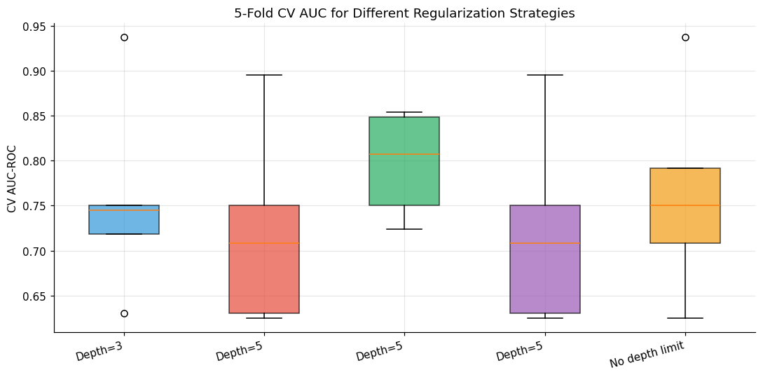
# Compare regularization strategies on the training set via 5-fold CV
cv = StratifiedKFold(n_splits=5, shuffle=True, random_state=42)

configs = {
    'Depth=3, no other constraints':
        DecisionTreeClassifier(max_depth=3, random_state=42),
    'Depth=5, no other constraints':
        DecisionTreeClassifier(max_depth=5, random_state=42),
    'Depth=5, min_samples_leaf=10':
        DecisionTreeClassifier(max_depth=5, min_samples_leaf=10, random_state=42),
    'Depth=5, min_impurity_decrease=0.01':
        DecisionTreeClassifier(max_depth=5, min_impurity_decrease=0.01, random_state=42),
    'No depth limit':
        DecisionTreeClassifier(random_state=42),
}

print(f"{'Configuration':<45} {'CV AUC (mean±std)'}")
print('─' * 65)
cv_results = {}
for name, clf in configs.items():
    scores = cross_val_score(clf, X_train, y_train, cv=cv, scoring='roc_auc')
    cv_results[name] = scores
    print(f"{name:<45} {scores.mean():.3f} ± {scores.std():.3f}")
Configuration                                 CV AUC (mean±std)
─────────────────────────────────────────────────────────────────
Depth=3, no other constraints                 0.756 ± 0.100
Depth=5, no other constraints                 0.722 ± 0.099
Depth=5, min_samples_leaf=10                  0.797 ± 0.052
Depth=5, min_impurity_decrease=0.01           0.722 ± 0.099
No depth limit                                0.762 ± 0.103
# Visualize the CV distributions
fig, ax = plt.subplots(figsize=(10, 5))
labels = list(cv_results.keys())
data   = [cv_results[k] for k in labels]
short_labels = [l.split(',')[0] for l in labels]

bp = ax.boxplot(data, patch_artist=True, notch=False, vert=True)
colors = ['#3498db','#e74c3c','#27ae60','#9b59b6','#f39c12']
for patch, color in zip(bp['boxes'], colors):
    patch.set_facecolor(color); patch.set_alpha(0.7)

ax.set_xticklabels(short_labels, rotation=15, ha='right')
ax.set_ylabel('CV AUC-ROC')
ax.set_title('5-Fold CV AUC for Different Regularization Strategies')
ax.grid(True, alpha=0.3)
plt.tight_layout(); plt.show()
🤔 Reflection 4.1 — Choosing Regularization#
min_samples_leafrequires each leaf to contain at least \(k\) training samples. Explain geometrically what this does to the decision boundary. How does it relate to the overfitting mechanism you diagnosed in Part 3? How does it relate to our in-class discussion on memorization vs. interpolation?min_impurity_decreaseprevents a split unless it reduces Gini by at least \(\delta\). This is a different kind of constraint than depth — it is adaptive rather than global. In what situation would this be preferable to setting max_depth?Look at the CV standard deviation across the five configurations. The no-depth-limit tree probably has high variance. Why? What does high variance in CV scores imply about deploying that model in a new hospital?
Preview: None of these regularization tricks fully solve the overfitting problem for a single tree. In a later lab, we’ll see that ensembles — particularly random forests and gradient boosting — address this more fundamentally. Before you get there: hypothesize how averaging 200 slightly different trees might produce better generalization than any one of them.
✅ Solution — Reflection 4.1#
1. min_samples_leaf=k prevents the tree from creating tiny leaf regions that contain fewer than \(k\) training samples. Geometrically, it ensures that every region of the feature space assigned a prediction contains at least \(k\) supporting examples. This directly addresses overfitting by preventing the tree from carving out regions for individual training points. It relates to memorization vs. generalization: with \(k=1\), a leaf can memorize a single sample; with \(k=10\), a leaf must represent a consensus of at least 10 samples.
2. min_impurity_decrease is adaptive because it prevents splits only when they don’t provide sufficient information gain. This is preferable to max_depth when different branches of the tree have different useful depths — one branch might benefit from going deep (because the data supports fine distinctions), while another should stop early (because further splitting just fits noise). Max_depth applies a uniform constraint; impurity decrease allows the tree to be deep where it helps and shallow where it doesn’t.
3. High CV variance means the model is very sensitive to which particular patients are in each fold. A model with AUC ranging from 0.65 to 0.88 across folds is unreliable — you can’t predict how it will perform at a new hospital. A model with consistent 0.78 ± 0.02 is more trustworthy, even if its average is slightly lower.
4. Averaging 200 slightly different trees might help because: each tree sees a different random subset of the training data (via bootstrap resampling) and makes different mistakes. If the mistakes are uncorrelated, averaging cancels out the noise. Mathematically, if each tree has variance \(\sigma^2\) and the trees are independent, the ensemble’s variance is \(\sigma^2/200\) — a massive reduction. The bias stays approximately the same (each tree is still a reasonable estimator), but variance drops dramatically. This is the core principle of bagging.
🧠 Final Reflection — Decision Trees as a Foundation#
Before moving on, answer these:
Bias-variance framing: A fully grown tree has low bias and high variance. A stump (depth=1) has high bias and low variance. Draw the bias-variance tradeoff curve for decision trees as a function of max_depth. Where does the optimal operating point land in our experiment?
The limits of a single tree: Even with optimal regularization, a single decision tree on our hard dataset achieves AUC ~0.78–0.83. What are the two fundamental reasons a single tree is limited? (Hint: one is about the partition it can represent, one is about sensitivity to training data.)
Clinical audit: A hospital wants to use a decision tree to decide which patients get expedited biopsy referrals. What are the two main arguments for using a tree over logistic regression in this context? What are the two main arguments against?
✅ Solution — Final Reflection#
1. A fully grown tree has low bias (it can represent any partition of the space, including the true one) and high variance (sensitive to training data). A stump has high bias (can only make one split — misses complex patterns) and low variance (robust to data perturbations). The bias-variance tradeoff curve as a function of depth: bias decreases monotonically, variance increases monotonically, and total error (bias² + variance) has a U-shape. The optimal depth in our experiment is around 3–5, where total error is minimized.
2. Two fundamental limitations of a single tree: (a) Representational limitation: the partition is axis-aligned and greedy (each split is locally optimal, not globally optimal), so the tree may need many splits to approximate a smooth boundary that a linear model captures in one step. (b) Instability: changing a few training samples can completely change the tree structure — the splits are discrete decisions, and a small change in data can flip a split threshold, cascading through the entire tree.
3. For using a tree: (a) complete transparency — the referral rule can be printed as “if smoothness > 0.1 and texture > 0.3, refer” which clinicians can audit and override; (b) no preprocessing required (trees handle raw feature values). Against: (a) inferior predictive performance — a single tree typically has lower AUC than logistic regression on tabular data; (b) instability — a slightly different training set could produce a completely different referral rule, undermining clinical trust.