
🔭 Lab 3: k-Nearest Neighbors#
BINF 4002 – Machine Learning for Health
Learning Objectives#
Understand KNN as a non-parametric, instance-based learner
Implement distance computation and majority voting yourself
Understand why feature scaling is critical for KNN — and more so than for trees
Explore the bias-variance tradeoff as \(k\) varies
Visualize and quantify the curse of dimensionality
Evaluate with decision curve analysis and compare to prior models
What is KNN — and How Does It Work?#
k-Nearest Neighbors is one of the conceptually simplest ML algorithms, and one of the most informative to understand deeply because it makes explicit assumptions that are hidden in other models.
The algorithm. Given a query point \(\mathbf{x}^*\), KNN:
Computes the distance from \(\mathbf{x}^*\) to every training point \(\mathbf{x}_i\)
Identifies the \(k\) training points with the smallest distances — the k nearest neighbors
Returns the majority class among those \(k\) neighbors as the prediction
Returns the fraction of the \(k\) neighbors with label 1 as the probability estimate
The most common distance is Euclidean distance: $\(d(\mathbf{a}, \mathbf{b}) = \|\mathbf{a} - \mathbf{b}\|_2 = \sqrt{\sum_{j=1}^d (a_j - b_j)^2}\)$
There is no training in the traditional sense — the model is just the stored training data. All computation happens at prediction time. This is why KNN is called a lazy learner or instance-based method.
Probability estimates are coarse. Because KNN votes among \(k\) neighbors, its probability output can only take values in \(\{0, 1/k, 2/k, \ldots, 1\}\) — a set of only \(k+1\) distinct values. For \(k=7\), that’s \(\{0, 0.14, 0.29, 0.43, 0.57, 0.71, 0.86, 1.0\}\). This discretization makes KNN probabilities poorly calibrated compared to logistic regression, which produces a continuous sigmoid output.
Why do we care about KNN in healthcare?
KNN is conceptually close to how clinicians reason: “Find patients similar to this one, and see what happened to them.” This is the basis of case-based reasoning — a formal methodology used in clinical decision support for decades. Modern EHR systems that surface “similar patients” for clinical comparison are implementing a form of nearest-neighbor retrieval. Understanding KNN deeply equips you to reason about the validity of those systems: What does “similar” mean? Which features define similarity? Does the similarity measure hold in high-dimensional EHR data? These are not abstract questions.
Dataset: Restricted breast cancer features (8 weakest features, 120 train samples) — the same hard split used in previous labs.
Set-up#
Upload data#
⚠️ First, upload processed_data.pkl from Lab 0 via the Files menu, or download it from the shared link.
import os

pkl_path = 'processed_data.pkl'
if os.path.exists(pkl_path):
    print("✅ Data File Found!")
else:
    raise FileNotFoundError(
        "processed_data.pkl not found! "
        "Make sure you have run Lab 0 (lab0_preprocessing.ipynb) in full and "
        "downloaded the output (or used the link above), and uploaded it here."
    )
✅ Data File Found!
Imports and Helpers#
import os, pickle, warnings
import numpy as np
import pandas as pd
import matplotlib.pyplot as plt
import matplotlib.gridspec as gridspec
import seaborn as sns
warnings.filterwarnings('ignore')

plt.rcParams['figure.dpi'] = 110
plt.rcParams['axes.spines.top'] = False
plt.rcParams['axes.spines.right'] = False
sns.set_palette("Set2")

pkl_path = 'processed_data.pkl'
if not os.path.exists(pkl_path):
    raise FileNotFoundError(
        "processed_data.pkl not found. Run Lab 0 first, or download from the link above "
        "and upload it here via the Files menu."
    )

with open(pkl_path, 'rb') as f:
    d = pickle.load(f)

X_train = d['X_train_hard']
y_train = d['y_train_hard']
X_val   = d['X_val_hard']
y_val   = d['y_val_hard']
X_test  = d['X_test_hard']
y_test  = d['y_test_hard']
feature_names = d['feature_names_hard']
class_names   = ['Malignant', 'Benign']

print(f"Train : {X_train.shape}  |  Val : {X_val.shape}  |  Test : {X_test.shape}")
print(f"Features: {feature_names}")
print(f"Class balance (train): {y_train.mean():.2f} benign, {1-y_train.mean():.2f} malignant")
Train : (100, 8)  |  Val : (114, 8)  |  Test : (114, 8)
Features: ['mean symmetry', 'compactness error', 'concavity error', 'smoothness error', 'texture error', 'fractal dimension error', 'symmetry error', 'mean fractal dimension']
Class balance (train): 0.60 benign, 0.40 malignant
from sklearn.neighbors import KNeighborsClassifier
from sklearn.metrics import confusion_matrix, roc_auc_score, roc_curve, auc

def print_metrics(y_true, y_pred, y_prob=None, label='Model'):
    tn,fp,fn,tp = confusion_matrix(y_true, y_pred).ravel()
    n = len(y_true)
    sens = tp/(tp+fn); spec = tn/(tn+fp)
    ppv  = tp/(tp+fp); npv  = tn/(tn+fn)
    prev = (tp+fn)/n
    print(f"{'─'*55}")
    print(f"  {label}")
    print(f"{'─'*55}")
    print(f"  Sensitivity  P(ŷ=1|y=1)  = {tp}/{tp+fn} = {sens:.3f}")
    print(f"  Specificity  P(ŷ=0|y=0)  = {tn}/{tn+fp} = {spec:.3f}")
    print(f"  PPV          P(y=1|ŷ=1)  = {tp}/{tp+fp} = {ppv:.3f}")
    print(f"  NPV          P(y=0|ŷ=0)  = {tn}/{tn+fn} = {npv:.3f}")
    print(f"  Prevalence               = {prev:.3f}")
    if y_prob is not None:
        auc_score = roc_auc_score(y_true, y_prob)
        print(f"  AUC-ROC                  = {auc_score:.3f}")
    print()

def decision_curve(y_true, y_prob, thresholds=None, label='Model', ax=None, color='#3498db'):
    """Net benefit decision curve. Net Benefit = TPR*prev - FPR*(1-prev)*t/(1-t)."""
    if thresholds is None:
        thresholds = np.linspace(0.01, 0.99, 150)
    prev = y_true.mean()
    nb_model, nb_all = [], []
    for t in thresholds:
        y_hat = (y_prob >= t).astype(int)
        tp = ((y_hat==1) & (y_true==1)).sum()
        fp = ((y_hat==1) & (y_true==0)).sum()
        n  = len(y_true)
        nb_model.append(tp/n - fp/n * t/(1-t))
        nb_all.append(prev - (1-prev)*t/(1-t))
    ax = ax or plt.gca()
    ax.plot(thresholds, nb_model, lw=2, label=label, color=color)
    ax.plot(thresholds, nb_all, 'k--', lw=1, alpha=0.5,
            label='Treat all' if label == 'Model' else '')
    ax.axhline(0, color='grey', lw=1, alpha=0.5)
    ax.set_xlabel('Probability Threshold'); ax.set_ylabel('Net Benefit')
    ax.set_ylim(-0.05, prev + 0.05)
    return np.array(nb_model)
Part 1 — Implement KNN from Scratch#
KNN is one of the simplest ML algorithms to implement, which makes it ideal for a “write it yourself” exercise. The entire model is three operations: compute distances, sort, vote.
Before coding: make sure you can trace through a small example by hand. Suppose \(k=3\), and the 3 nearest neighbors of a query point have labels \([0, 1, 1]\). The majority class is 1 (Benign), and the probability estimate is \(2/3 \approx 0.67\).
Notice that this probability can only take values in \(\{0, 1/3, 2/3, 1\}\) — three distinct values for \(k=3\). This discretization is a fundamental limitation of KNN’s probability estimates that we’ll revisit in Part 3.
# ── SOLUTION ──────────────────────────────────────────────────────────────────
# Implement KNN prediction for a single query point.

def euclidean_distance(a, b):
    """
    Euclidean distance between two vectors: sqrt(sum((a_i - b_i)^2))
    Both a and b are 1-D numpy arrays of the same length.
    """
    return np.sqrt(np.sum((a - b) ** 2))


def knn_predict_one(X_train, y_train, x_query, k):
    """
    Predict the class for a single query point using KNN.
    Steps:
      1. Compute distances from x_query to all training points
      2. Find the k nearest neighbors (smallest distances)
      3. Majority vote among their labels
      4. Return (predicted_class, probability_of_class_1)
         where probability = fraction of the k neighbors with label=1
    """
    # Step 1: distances to all training points
    distances = np.array([euclidean_distance(x_query, x_i) for x_i in X_train])

    # Step 2: indices of k nearest neighbors (sorted by ascending distance)
    nn_indices = np.argsort(distances)[:k]

    # Step 3: labels of those k neighbors
    nn_labels  = y_train[nn_indices]

    # Step 4: fraction with label=1 → class prediction
    prob_1 = nn_labels.mean()
    pred   = int(prob_1 >= 0.5)
    return pred, prob_1


def knn_predict(X_train, y_train, X_query, k):
    """Predict for a batch of query points (calls knn_predict_one in a loop)."""
    preds, probs = [], []
    for x in X_query:
        pred, prob = knn_predict_one(X_train, y_train, x, k)
        preds.append(pred); probs.append(prob)
    return np.array(preds), np.array(probs)
# ── Sanity check — run this after implementing above ──────────────────────────
k_test = 7
knn_sk = KNeighborsClassifier(n_neighbors=k_test, metric='euclidean')
knn_sk.fit(X_train, y_train)

your_preds, your_probs = knn_predict(X_train, y_train, X_val[:20], k_test)
sk_preds   = knn_sk.predict(X_val[:20])
sk_probs   = knn_sk.predict_proba(X_val[:20])[:, 1]

max_prob_diff = np.abs(your_probs - sk_probs).max()
n_agree = (your_preds == sk_preds).sum()

assert n_agree == 20, (
    f"Predictions disagree on {20-n_agree}/20 samples. "
    "Check your argsort direction — smaller distance = nearer neighbor."
)
assert max_prob_diff < 1e-9, (
    f"Probabilities differ by up to {max_prob_diff:.2e}. "
    "Check that you're computing nn_labels.mean(), not sum."
)
print(f"✓ All 20 predictions match sklearn (max prob diff = {max_prob_diff:.2e})")
print()
print(f"{'Val sample':<12} {'True label':<14} {'Your prob':>10} {'sk prob':>10} {'Match':>8}")
print("─" * 60)
for i in range(8):
    match = "✓" if your_preds[i] == sk_preds[i] else "✗"
    print(f"  Val[{i}]     {class_names[y_val[i]]:<14} {your_probs[i]:>10.3f} {sk_probs[i]:>10.3f} {match:>8}")
✓ All 20 predictions match sklearn (max prob diff = 0.00e+00)

Val sample   True label      Your prob    sk prob    Match
────────────────────────────────────────────────────────────
  Val[0]     Benign              0.857      0.857        ✓
  Val[1]     Benign              0.571      0.571        ✓
  Val[2]     Benign              0.714      0.714        ✓
  Val[3]     Malignant           0.286      0.286        ✓
  Val[4]     Benign              0.286      0.286        ✓
  Val[5]     Benign              0.857      0.857        ✓
  Val[6]     Benign              1.000      1.000        ✓
  Val[7]     Benign              0.429      0.429        ✓
🤔 Reflection 1.1 — The KNN Algorithm#
Your
knn_predictfunction loops over query points, and for each one computes distances to all \(n_{\text{train}}\) training points, each of which requires \(d\) subtractions and additions. What is the time complexity of predicting on \(n_{\text{test}}\) samples? How does this compare to logistic regression’s prediction complexity? What happens at \(n_{\text{train}} = 10^6\) (a typical EHR cohort)?With \(k=1\), your implementation will always return the exact training label for any training point (distance = 0 to itself). Is this “overfitting” in the same sense as a deep decision tree? How does the failure mode differ? (Hint: a decision tree’s overfitting reflects the learned parameters; KNN’s reflects the stored data.)
The probability output of KNN can only take values \(\{0, 1/k, 2/k, \ldots, 1\}\) — just \(k+1\) distinct values. For \(k=7\), the finest probability distinction you can make is \(1/7 \approx 0.14\). Why does this matter for a decision curve, where clinical decisions are sensitive to thresholds like \(t=0.10\) vs \(t=0.15\)?
KNN treats all features as equally important when computing distances. Logistic regression and trees both learn which features matter. What does this imply about KNN’s sensitivity to irrelevant features? How does this connect to the noise-feature experiment you’ll see in Part 4?
✅ Solution — Reflection 1.1#
1. Time complexity: for each of \(n_{\text{test}}\) query points, we compute distances to all \(n_{\text{train}}\) points (\(O(d)\) per distance), then sort (\(O(n_{\text{train}} \log n_{\text{train}})\)). Total: \(O(n_{\text{test}} \cdot n_{\text{train}} \cdot d)\). Logistic regression prediction is just \(O(n_{\text{test}} \cdot d)\) — a single dot product per sample. At \(n_{\text{train}} = 10^6\), KNN must compute a million distances per query point, making it extremely slow for real-time clinical applications without approximate nearest neighbor methods.
2. With \(k=1\), the nearest neighbor of any training point is itself (distance = 0), so training accuracy is always 100%. This is “overfitting” in a different sense than a deep decision tree: the tree encodes overfit structure in its learned thresholds, while KNN’s overfit is in the stored data itself. The failure mode is that a single noisy training point directly corrupts predictions for its neighborhood — there’s no parameter to regularize, only \(k\) to increase.
3. With \(k=7\), probabilities can only be \(\{0, 1/7, 2/7, 3/7, 4/7, 5/7, 6/7, 1\}\) — gaps of 0.143. For a clinical threshold like \(t=0.10\), the model has no predictions between 0 and 0.143 — so it either predicts 0 (definitely no treatment) or ≥0.143 (treatment). It cannot make fine-grained distinctions in the 0.10–0.15 range that DCA requires. This creates the “staircase” DCA curves we’ll see later.
4. KNN treats all features equally in the distance computation. If 7 of 8 features are noise, the noise dominates the distance, and the “nearest neighbors” are determined mostly by random noise dimensions rather than the one informative feature. Logistic regression can learn to assign near-zero weight to irrelevant features; trees simply won’t split on uninformative features. KNN has no such mechanism — it must use all features equally.
Part 2 — Why Feature Scaling Is Critical for KNN#
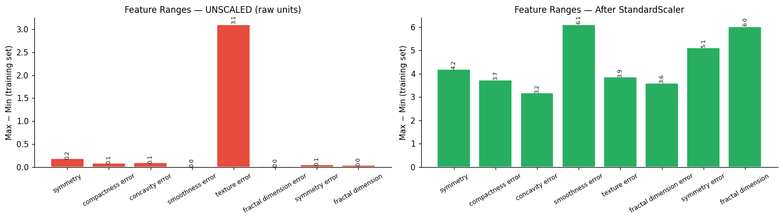
In Lab 0, you saw that the 8 restricted features have very different raw scales — some measured in fractions, some in hundreds. For decision trees, this doesn’t matter: splits are on individual features, so absolute scale is irrelevant. For logistic regression, predictions don’t change (only coefficient interpretability does).
For KNN, scale is everything. The Euclidean distance is a sum across all features: $\(d(\mathbf{a}, \mathbf{b})^2 = \sum_{j=1}^d (a_j - b_j)^2\)$
A feature with range 1000 contributes up to \(1000^2 = 10^6\) to this sum. A feature with range 1 contributes at most 1. The high-range feature completely dominates who is “nearest.” This is not a choice — it is a mathematical fact about Euclidean distance.
Question: How does this challenge manifest with other distance metrics?
We demonstrate this below using actual unscaled feature values reconstructed from the original breast cancer dataset.
from sklearn.datasets import load_breast_cancer
from sklearn.model_selection import train_test_split
from sklearn.preprocessing import StandardScaler

# Reconstruct unscaled hard splits (same random seed and indices as Lab 0)
bc      = load_breast_cancer()
hard_idx = d['hard_col_idx']           # indices of the 8 restricted features in the full 30

X_bc_hard = bc.data[:, hard_idx]
y_bc      = bc.target

# Replicate Lab 0 split structure: 60/20/20 stratified, then subsample train to 120
X_tr_r, X_tmp_r, y_tr_r, y_tmp_r = train_test_split(
    X_bc_hard, y_bc, test_size=0.40, random_state=42, stratify=y_bc)
X_v_r, X_te_r, y_v_r, y_te_r = train_test_split(
    X_tmp_r, y_tmp_r, test_size=0.50, random_state=42, stratify=y_tmp_r)

rng = np.random.default_rng(42)
sidx = rng.choice(len(X_tr_r), 120, replace=False)
X_train_raw, y_train_raw = X_tr_r[sidx], y_tr_r[sidx]
X_val_raw                = X_v_r

# --- Feature range comparison ---
ranges_raw    = X_train_raw.max(0) - X_train_raw.min(0)
ranges_scaled = X_train.max(0)     - X_train.min(0)

fig, axes = plt.subplots(1, 2, figsize=(14, 4))
short_names = [f.replace('mean ','').replace('worst ','') for f in feature_names]

for ax, vals, title, color in zip(
    axes,
    [ranges_raw, ranges_scaled],
    ['Feature Ranges — UNSCALED (raw units)', 'Feature Ranges — After StandardScaler'],
    ['#e74c3c', '#27ae60']
):
    bars = ax.bar(short_names, vals, color=color, edgecolor='white', linewidth=1.2)
    ax.set_title(title, fontsize=11); ax.tick_params(axis='x', rotation=30, labelsize=8)
    ax.set_ylabel('Max − Min (training set)')
    for bar, val in zip(bars, vals):
        ax.text(bar.get_x()+bar.get_width()/2, bar.get_height()*1.01,
                f'{val:.1f}', ha='center', fontsize=7, rotation=90)

plt.tight_layout(); plt.show()
# AUC comparison: KNN with and without scaling
k_demo = 7

knn_scaled   = KNeighborsClassifier(n_neighbors=k_demo, metric='euclidean')
knn_unscaled = KNeighborsClassifier(n_neighbors=k_demo, metric='euclidean')
knn_scaled.fit(X_train, y_train)
knn_unscaled.fit(X_train_raw, y_train_raw)

auc_scaled   = roc_auc_score(y_val, knn_scaled.predict_proba(X_val)[:,1])
auc_unscaled = roc_auc_score(y_val, knn_unscaled.predict_proba(X_val_raw)[:,1])

print(f"KNN (k={k_demo}) — SCALED features  : AUC = {auc_scaled:.3f}")
print(f"KNN (k={k_demo}) — UNSCALED features: AUC = {auc_unscaled:.3f}")
print(f"\nAUC drop from not scaling: {auc_scaled - auc_unscaled:.3f}")
KNN (k=7) — SCALED features  : AUC = 0.780
KNN (k=7) — UNSCALED features: AUC = 0.564

AUC drop from not scaling: 0.216
# Visualize HOW neighbors change: pick a query point and show its 7 nearest
# neighbors in scaled vs. unscaled space (projected onto 2 features for visualization)

query_idx = 4   # pick a validation patient

# Use two features that differ most in scale: pick highest-range vs lowest-range raw
raw_hi_idx = int(np.argmax(ranges_raw))    # dominates unscaled distance
raw_lo_idx = int(np.argmin(ranges_raw))    # barely contributes unscaled

# Find k nearest neighbors in each space
k_vis = 7
from sklearn.neighbors import NearestNeighbors

nn_scaled   = NearestNeighbors(n_neighbors=k_vis+1).fit(X_train)
nn_unscaled = NearestNeighbors(n_neighbors=k_vis+1).fit(X_train_raw)

# Distances and indices (skip self if present)
_, idx_sc  = nn_scaled.kneighbors(X_val[[query_idx]])
_, idx_un  = nn_unscaled.kneighbors(X_val_raw[[query_idx]])
idx_sc, idx_un = idx_sc[0][:k_vis], idx_un[0][:k_vis]

fig, axes = plt.subplots(1, 2, figsize=(14, 5))
data_and_labels_pairs = [(X_train_raw, y_train_raw, X_val_raw), (X_train, y_train, X_val)]
titles = ['UNSCALED (dominated by high-range feature)', 'SCALED (both features contribute equally)']
nn_idx_pairs = [idx_un, idx_sc]

for ax, (Xtr, ytr, Xv), nn_idx, title in zip(axes, data_and_labels_pairs, nn_idx_pairs, titles):
    # All training points
    for cls, color, marker in [(0,'#e74c3c','o'), (1,'#27ae60','s')]:
        mask = ytr == cls
        ax.scatter(Xtr[mask, raw_hi_idx], Xtr[mask, raw_lo_idx],
                   c=color, marker=marker, alpha=0.3, s=25, label=class_names[cls])
    # k nearest neighbors
    ax.scatter(Xtr[nn_idx, raw_hi_idx], Xtr[nn_idx, raw_lo_idx],
               c='#f39c12', s=120, zorder=5, edgecolors='black', linewidths=1.5,
               label=f'{k_vis} nearest neighbors')
    # Query point
    ax.scatter(Xv[query_idx, raw_hi_idx], Xv[query_idx, raw_lo_idx],
               c='#9b59b6', s=200, marker='*', zorder=6, label='Query patient')
    ax.set_xlabel(feature_names[raw_hi_idx] + ' (high range)')
    ax.set_ylabel(feature_names[raw_lo_idx] + ' (low range)')
    ax.set_title(title, fontsize=10); ax.legend(fontsize=8)

plt.suptitle(f'How Scaling Changes the {k_vis} Nearest Neighbors of Val[{query_idx}]',
             fontsize=11, y=1.02)
plt.tight_layout(); plt.show()

# Show what the scaled and unscaled neighborhoods voted
nn_votes_sc = y_train[idx_sc]
nn_votes_un = y_train_raw[idx_un]
print(f"Scaled   neighborhood labels: {nn_votes_sc.tolist()} \u2192 pred={int(nn_votes_sc.mean()>=0.5)}, prob={nn_votes_sc.mean():.2f}")
print(f"Unscaled neighborhood labels: {nn_votes_un.tolist()} \u2192 pred={int(nn_votes_un.mean()>=0.5)}, prob={nn_votes_un.mean():.2f}")
print(f"True label: {class_names[y_val[query_idx]]}")
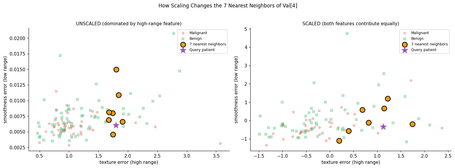
Scaled   neighborhood labels: [1, 1, 0, 0, 0, 0, 0] → pred=0, prob=0.29
Unscaled neighborhood labels: [1, 1, 0, 0, 1, 0, 1] → pred=1, prob=0.57
True label: Benign
🤔 Reflection 2.1 — Scaling, Distance, and Clinical Variables#
In the visualization above, the unscaled nearest neighbors cluster along the high-range feature axis, ignoring the low-range feature almost entirely. Now look at the AUC numbers. Does the lower-range feature contain useful information that the unscaled model is discarding? How would you test this?
StandardScaler normalizes each feature to zero mean and unit variance. But is standardized Euclidean distance always the right distance for clinical data? Consider a feature like “number of hospitalizations in the past year” (integer, heavily right-skewed) or binary comorbidity flags (0/1). Is Euclidean distance sensible for these? What would you use instead?
Suppose you deploy a scaled KNN model and a new hospital feeds in data where one feature is measured in different units (e.g., serum creatinine in µmol/L instead of mg/dL). The scaler you trained on won’t know about this. What happens to that feature’s contribution to distances? How would you detect this failure in production?
Mahalanobis distance accounts for correlations between features: \(d_M(\mathbf{a}, \mathbf{b}) = \sqrt{(\mathbf{a}-\mathbf{b})^T \Sigma^{-1} (\mathbf{a}-\mathbf{b})}\) where \(\Sigma\) is the feature covariance matrix. In Lab 0 we saw that several features are nearly perfectly correlated (r > 0.99). How would Mahalanobis distance treat these correlated features differently than Euclidean distance? When would this matter clinically?
High-dimensionality Here, we have a low-dimensional dataset, but in many settings (and with the real, full dataset we could use here), we could have many more features. What problems do \(k\)-nns face in high dimensions? Hint: Recall our discussion on the differences between low and high dimensional spaces in the calculus and optimization lecture.
Bonus: Optimal Distance Metric? What is the “optimal” distance metric to use for a \(k\)-nn model for a given task? Why don’t we use that?
✅ Solution — Reflection 2.1#
1. Yes — the lower-range feature does contain useful information. You can test this by running KNN on each feature individually and comparing AUC. Even if the AUC of the low-range feature alone is modest, it contributes to discrimination. The unscaled model discards this information because the high-range feature’s distance contribution overwhelms it.
2. Standardized Euclidean distance isn’t always appropriate. For integer-valued counts (hospitalizations), the Euclidean difference between 0 and 1 is as large as between 5 and 6, which may not reflect clinical similarity. For binary flags, Euclidean distance reduces to Hamming-like counting. Better alternatives: Manhattan distance for sparse/count data, Gower distance for mixed types, or learned distance metrics (Mahalanobis, or metric learning methods like LMNN).
3. If one feature is in µmol/L instead of mg/dL (conversion factor ~88.4 for creatinine), the scaler trained on mg/dL will produce incorrect standardized values — the feature will appear to have extreme values. This would massively distort KNN distances. Detection: monitor input feature distributions in production and flag when a feature’s distribution deviates significantly from the training distribution (e.g., using a KS test or comparing means/variances).
4. Mahalanobis distance down-weights correlated features by using the inverse covariance matrix \(\Sigma^{-1}\). If two features have r=0.99, Mahalanobis effectively treats them as one degree of freedom (differences along the correlated direction are discounted), while Euclidean treats them as two independent dimensions (double-counting the same information). This matters when many lab values reflect the same underlying physiology (e.g., kidney function markers).
5. In high dimensions, KNN suffers from the curse of dimensionality: all pairwise distances concentrate near the same value, so “nearest” and “farthest” neighbors become nearly equidistant. The distinction between neighbors collapses, making the \(k\)-nearest neighbor selection essentially random. The volume of a hypersphere grows exponentially, so to maintain a fixed number of neighbors within a fixed distance, you need exponentially more data.
6. (Bonus) The “optimal” distance metric for a \(k\)-NN classification task would be one that places points of the same class close together and different classes far apart. This is exactly what metric learning methods (like Large Margin Nearest Neighbors, LMNN) try to learn. We don’t use it by default because (a) it requires labeled data to learn the metric, (b) it adds complexity and hyperparameters, and (c) with small sample sizes, learning a distance metric can itself overfit.
Part 3 — Bias-Variance Tradeoff as \(k\) Varies#
The hyperparameter \(k\) directly controls the bias-variance tradeoff:
\(k=1\): The model predicts the label of the single nearest training point. The decision boundary is highly irregular — it perfectly fits every training example (training accuracy = 100%) but is very sensitive to individual noisy points. This is low bias, high variance.
\(k = n_{\text{train}}\): Every query point gets the same prediction — the majority class across all training data. The model ignores the query entirely. This is maximum bias, zero variance.
\(k = k^*\) (optimal): Balances these extremes by averaging over enough neighbors to smooth out noise, but not so many that local structure is lost.
Unlike decision trees where the bias-variance tradeoff is controlled by depth (a discrete structural parameter), in KNN it’s controlled by \(k\) — a continuous smoothing parameter that acts directly on the prediction rule.
k_values = list(range(1, 51))
train_accs, val_accs, val_aucs = [], [], []

for k in k_values:
    knn = KNeighborsClassifier(n_neighbors=k)
    knn.fit(X_train, y_train)
    train_accs.append(knn.score(X_train, y_train))
    val_accs.append(knn.score(X_val, y_val))
    val_aucs.append(roc_auc_score(y_val, knn.predict_proba(X_val)[:,1]))

best_k   = k_values[np.argmax(val_aucs)]
best_auc = max(val_aucs)

fig, axes = plt.subplots(1, 2, figsize=(14, 5))

axes[0].plot(k_values, train_accs, 'o-', color='#3498db', lw=1.5, markersize=4, label='Train accuracy')
axes[0].plot(k_values, val_accs,   's-', color='#e74c3c', lw=1.5, markersize=4, label='Val accuracy')
axes[0].axvline(best_k, color='grey', linestyle='--', alpha=0.8, label=f'Best k={best_k} (by AUC)')
axes[0].fill_between(k_values, train_accs, val_accs, alpha=0.1, color='orange', label='Overfit gap')
axes[0].set_xlabel('k (number of neighbors)'); axes[0].set_ylabel('Accuracy')
axes[0].set_title('Bias-Variance Tradeoff in KNN\n(left=high variance; right=high bias)')
axes[0].legend(fontsize=9); axes[0].grid(True, alpha=0.3)
# Annotations
axes[0].annotate('High variance\n(k=1: train=100%)', xy=(1, train_accs[0]),
                  xytext=(6, 0.92), arrowprops=dict(arrowstyle='->', color='#3498db'),
                  fontsize=8, color='#3498db')
axes[0].annotate('High bias\n(k=50: predicts majority)', xy=(50, val_accs[-1]),
                  xytext=(35, 0.6), arrowprops=dict(arrowstyle='->', color='#e74c3c'),
                  fontsize=8, color='#e74c3c')

axes[1].plot(k_values, val_aucs, 'o-', color='#9b59b6', lw=2, markersize=5)
axes[1].axvline(best_k, color='grey', linestyle='--', alpha=0.8, label=f'Best k={best_k} (AUC={best_auc:.3f})')
axes[1].set_xlabel('k'); axes[1].set_ylabel('Validation AUC-ROC')
axes[1].set_title('KNN Validation AUC vs k'); axes[1].legend(); axes[1].grid(True, alpha=0.3)

plt.tight_layout(); plt.show()

print(f"k=1         : train={train_accs[0]:.3f}  val_acc={val_accs[0]:.3f}  val_auc={val_aucs[0]:.3f}")
print(f"k={best_k:<2} (best)  : train={train_accs[best_k-1]:.3f}  val_acc={val_accs[best_k-1]:.3f}  val_auc={val_aucs[best_k-1]:.3f}")
print(f"k={len(X_train)} (=n_train): train={train_accs[-1]:.3f}  val_acc={val_accs[-1]:.3f}  val_auc={val_aucs[-1]:.3f}")
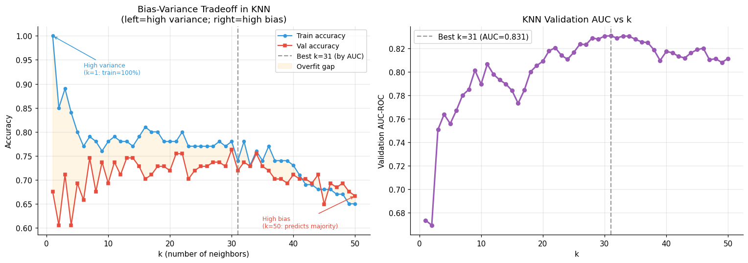
k=1         : train=1.000  val_acc=0.675  val_auc=0.674
k=31 (best)  : train=0.740  val_acc=0.719  val_auc=0.831
k=100 (=n_train): train=0.650  val_acc=0.667  val_auc=0.812
The Coarseness of KNN Probability Estimates#
Before the reflection, let’s directly visualize the discretization problem mentioned in the intro — KNN probabilities can only take \(k+1\) distinct values.
# Calibration comparison: KNN vs Logistic Regression
# Does KNN's coarse probability output hurt calibration?
from sklearn.linear_model import LogisticRegression
from sklearn.calibration import calibration_curve

best_knn_tmp = KNeighborsClassifier(n_neighbors=best_k).fit(X_train, y_train)
lr_tmp       = LogisticRegression(C=1.0, max_iter=1000, random_state=42).fit(X_train, y_train)

knn_probs = best_knn_tmp.predict_proba(X_val)[:,1]
lr_probs  = lr_tmp.predict_proba(X_val)[:,1]

fig, axes = plt.subplots(1, 2, figsize=(14, 5))

# Histogram of predicted probabilities
axes[0].hist(lr_probs,  bins=30, alpha=0.6, color='#3498db', label='Logistic Regression (continuous)')
axes[0].hist(knn_probs, bins=np.linspace(0, 1, best_k+2)-0.5/(best_k), alpha=0.6,
             color='#e67e22', label=f'KNN k={best_k} ({best_k+1} possible values)')
axes[0].set_xlabel('Predicted Probability P(Benign)')
axes[0].set_ylabel('Count'); axes[0].set_title('Distribution of Predicted Probabilities')
axes[0].legend(fontsize=9)
# Mark discrete KNN values
for v in np.arange(0, best_k+1)/best_k:
    axes[0].axvline(v, color='#e67e22', lw=0.7, alpha=0.4)

# Calibration curves (reliability diagrams)
# Note: with small val set these will be noisy — the shape matters more than exact values
try:
    frac_pos_knn, mean_pred_knn = calibration_curve(y_val, knn_probs, n_bins=5, strategy='quantile')
    frac_pos_lr,  mean_pred_lr  = calibration_curve(y_val, lr_probs,  n_bins=5, strategy='quantile')
    axes[1].plot(mean_pred_knn, frac_pos_knn, 'o-', color='#e67e22', lw=2, label=f'KNN k={best_k}')
    axes[1].plot(mean_pred_lr,  frac_pos_lr,  's-', color='#3498db', lw=2, label='Logistic Regression')
    axes[1].plot([0,1],[0,1], 'k--', lw=1, label='Perfect calibration')
    axes[1].set_xlabel('Mean predicted probability'); axes[1].set_ylabel('Fraction actually positive')
    axes[1].set_title('Calibration Curves (Reliability Diagram)\n(closer to diagonal = better calibrated)')
    axes[1].legend(fontsize=9); axes[1].grid(True, alpha=0.3)
except Exception as e:
    axes[1].text(0.5, 0.5, f'Calibration plot requires more data\n({e})',
                 ha='center', va='center', transform=axes[1].transAxes)

plt.tight_layout(); plt.show()
print(f"\nKNN (k={best_k}) possible probability values: {[round(i/best_k,3) for i in range(best_k+1)]}")
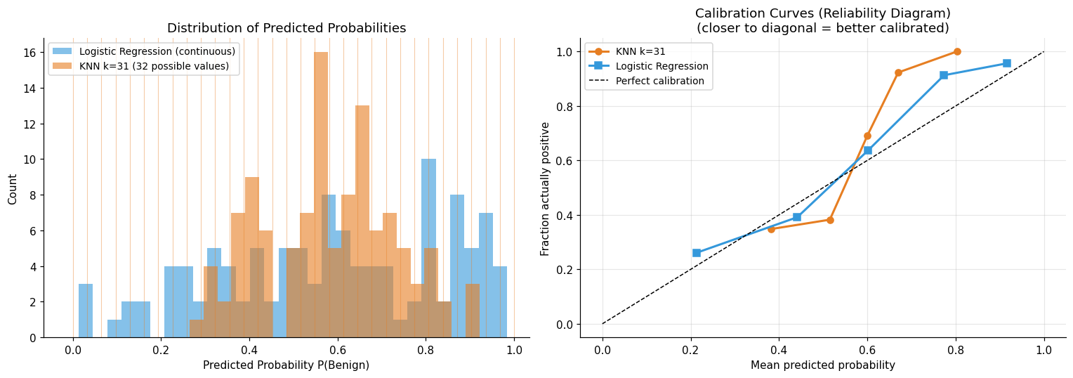
KNN (k=31) possible probability values: [0.0, 0.032, 0.065, 0.097, 0.129, 0.161, 0.194, 0.226, 0.258, 0.29, 0.323, 0.355, 0.387, 0.419, 0.452, 0.484, 0.516, 0.548, 0.581, 0.613, 0.645, 0.677, 0.71, 0.742, 0.774, 0.806, 0.839, 0.871, 0.903, 0.935, 0.968, 1.0]
🤔 Reflection 3.1 — Bias-Variance in KNN#
At \(k=1\), training accuracy is 100%. Explain why this is always guaranteed for KNN with \(k=1\), regardless of the training data. Is this “overfitting” in the same sense as a depth-20 decision tree? (Hint: a decision tree’s overfit is encoded in learned thresholds; what is KNN’s overfit encoded in?)
At \(k = n_{\text{train}}\) (here \(k=120\)), what is the prediction for every single query point, and what is the corresponding training and validation accuracy? Express the bias of this classifier in terms of the class prevalence.
The optimal \(k\) we found (printed by the code above) was selected by validation AUC. If we doubled the training set to 240 samples, would you expect the optimal \(k\) to increase, decrease, or stay the same? Give a principled argument — think about what \(k\) controls controlling geometrically as \(n_{\text{train}}\) grows.
KNN stores all training data and has no learned parameters. What are the concrete implications for: (a) memory when \(n_{\text{train}} = 10^6\), (b) prediction latency under a 100ms SLA, (c) incorporating a new labeled patient without retraining? For (b), look up “k-d trees” and “ball trees” — what do they provide? For (c), look up “k-d trees” and “ball trees” — what do they provide?
Look at the calibration plot. The KNN probabilities can only fall on \(\{{i/k : i = 0, \ldots, k\}}\). Concretely, for \(kyour best \) (printed above), what is the smallest probability difference the model can distinguish? Why does this matter when a clinical guideline says “refer if risk > 20%”?
✅ Solution — Reflection 3.1#
1. At \(k=1\), training accuracy is always 100% because each training point is its own nearest neighbor (distance = 0). This is guaranteed regardless of the data. It’s overfitting in the sense that the model memorizes every training point, but unlike a decision tree (where overfit is encoded in learned split thresholds), KNN’s “overfit” is encoded in the stored data itself. There are no parameters to regularize — the data is the model.
2. At \(k = n_{\text{train}} = 100\), every query point gets the same prediction: the majority class across all training data. If 63% of training samples are benign, the model predicts P(benign) = 0.63 for every patient. Training accuracy = fraction of samples matching the majority class. The bias is \(|P(\text{majority}) - \text{optimal threshold}|\) — the model completely ignores the input features.
3. If we doubled the training set to 200 samples, the optimal \(k\) would likely increase. With more data, the local density of training points increases — each neighborhood is more populated, so you can average over more neighbors without losing local structure. Geometrically, the number of neighbors within a fixed radius grows with \(n_{\text{train}}\), so you can afford a larger \(k\) before the neighborhood becomes too large and crosses class boundaries.
4. (a) Memory: at \(n_{\text{train}} = 10^6\) with 8 float64 features, storing the training set requires ~61 MB — manageable, but grows linearly with \(n\). (b) Prediction latency: computing distances to \(10^6\) points takes ~10ms per query on modern hardware, but this scales linearly and doesn’t meet a 100ms SLA for batch predictions. K-d trees and ball trees provide \(O(\log n)\) average-case query time by pre-indexing the training data in a spatial tree structure. (c) Adding a new patient: KNN can incorporate new data by simply appending it to the training set — no retraining needed. This is a significant advantage over parametric models that must be refitted.
5. For the best \(k\) found (printed above), the smallest probability difference is \(1/k\). For example, if \(k=7\), the model cannot distinguish between risks of 0.14 and 0.28 — it can only output multiples of 0.143. If a clinical guideline says “refer if risk > 20%,” the model can only say “14% (no refer)” or “29% (refer)” — it cannot identify the 20% boundary. This coarseness is a fundamental limitation of KNN probability estimates.
Part 4 — Curse of Dimensionality#
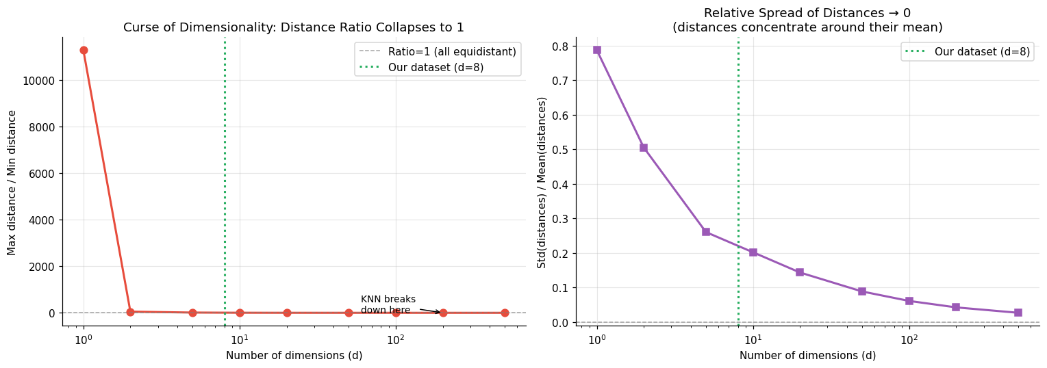
In high dimensions, nearest neighbors are no longer meaningfully “near.” All pairwise distances converge to approximately the same value, so the distinction between the “nearest” and “farthest” neighbor collapses. This is the curse of dimensionality, first described by Bellman (1957) and a fundamental problem for any distance-based method. Recall we discussed this in the Calculus and Optimization Lecture.
Why does this happen? In \(d\) dimensions, a random point drawn from \(\mathcal{N}(0, I_d)\) has squared distance \(\sum_{j=1}^d Z_j^2\) from the origin, where \(Z_j \sim N(0,1)\). By the law of large numbers, this sum concentrates near \(d\) as \(d \to \infty\), with standard deviation \(\sqrt{2d}\). The ratio of std to mean scales as \(1/\sqrt{d} \to 0\), meaning all distances become increasingly similar relative to their magnitude.
In practice this means: with 500 EHR features, the 1st nearest neighbor and the 500th nearest neighbor are almost equidistant from a query point. “Nearest” becomes meaningless.
# Demonstrate: as dimensionality grows, max/min distance ratio converges to 1
dims = [1, 2, 5, 10, 20, 50, 100, 200, 500]
rng_cod = np.random.default_rng(42)

min_dists, max_dists, ratios, rel_stds = [], [], [], []

print(f"{'Dims':>6} {'Min dist':>10} {'Max dist':>10} {'Max/Min':>10} {'Std/Mean':>10}")
print("─" * 52)
for d in dims:
    pts   = rng_cod.standard_normal((1000, d))
    query = pts[0:1]
    dists = np.sqrt(((pts[1:] - query)**2).sum(axis=1))
    mn, mx, std, mean = dists.min(), dists.max(), dists.std(), dists.mean()
    min_dists.append(mn); max_dists.append(mx)
    ratios.append(mx/mn); rel_stds.append(std/mean)
    print(f"{d:>6} {mn:>10.3f} {mx:>10.3f} {mx/mn:>10.3f} {std/mean:>10.3f}")
  Dims   Min dist   Max dist    Max/Min   Std/Mean
────────────────────────────────────────────────────
     1      0.000      3.953  11283.350      0.788
     2      0.075      3.857     51.651      0.505
     5      0.610      7.083     11.610      0.261
    10      1.753      7.861      4.484      0.202
    20      3.411      8.608      2.524      0.144
    50      7.043     12.400      1.761      0.089
   100     11.213     17.271      1.540      0.061
   200     17.318     22.697      1.311      0.043
   500     27.975     34.636      1.238      0.027
# Visualize the convergence
fig, axes = plt.subplots(1, 2, figsize=(14, 5))

axes[0].plot(dims, ratios, 'o-', color='#e74c3c', lw=2, markersize=7)
axes[0].axhline(1.0, color='grey', linestyle='--', lw=1, alpha=0.7, label='Ratio=1 (all equidistant)')
axes[0].set_xlabel('Number of dimensions (d)'); axes[0].set_ylabel('Max distance / Min distance')
axes[0].set_title('Curse of Dimensionality: Distance Ratio Collapses to 1')
axes[0].set_xscale('log'); axes[0].grid(True, alpha=0.3); axes[0].legend()
axes[0].annotate('KNN breaks\ndown here', xy=(200, ratios[dims.index(200)]),
                  xytext=(60, ratios[dims.index(200)]+0.3),
                  arrowprops=dict(arrowstyle='->', color='black'), fontsize=9)

axes[1].plot(dims, rel_stds, 's-', color='#9b59b6', lw=2, markersize=7)
axes[1].axhline(0, color='grey', linestyle='--', lw=1, alpha=0.7)
axes[1].set_xlabel('Number of dimensions (d)')
axes[1].set_ylabel('Std(distances) / Mean(distances)')
axes[1].set_title('Relative Spread of Distances → 0\n(distances concentrate around their mean)')
axes[1].set_xscale('log'); axes[1].grid(True, alpha=0.3)

# Mark our actual dataset
axes[0].axvline(8, color='#27ae60', linestyle=':', lw=2, label='Our dataset (d=8)')
axes[0].legend()
axes[1].axvline(8, color='#27ae60', linestyle=':', lw=2, label='Our dataset (d=8)')
axes[1].legend()

plt.tight_layout(); plt.show()
# AUC degradation as random noise features are added
print("KNN AUC as irrelevant noise features are added:")
print(f"{'Noise features':>15} {'Total d':>10} {'Val AUC':>10}  Note")
print("─" * 55)

noise_levels = [0, 2, 5, 10, 20, 50, 100]
noise_aucs   = []

for n_noise in noise_levels:
    rng_n = np.random.default_rng(0)
    Xtr_n = np.hstack([X_train, rng_n.standard_normal((len(X_train), n_noise))])
    Xv_n  = np.hstack([X_val,   rng_n.standard_normal((len(X_val),   n_noise))])
    knn_n = KNeighborsClassifier(n_neighbors=best_k)
    knn_n.fit(Xtr_n, y_train)
    auc_n = roc_auc_score(y_val, knn_n.predict_proba(Xv_n)[:,1])
    noise_aucs.append(auc_n)
    note = " ← baseline" if n_noise == 0 else (" ← collapses" if n_noise == 100 else "")
    print(f"{n_noise:>15} {8+n_noise:>10} {auc_n:>10.3f}{note}")

fig, ax = plt.subplots(figsize=(9, 4))
ax.plot(noise_levels, noise_aucs, 'o-', color='#e74c3c', lw=2, markersize=7)
ax.axhline(noise_aucs[0], color='grey', linestyle='--', lw=1, label=f'Baseline AUC (d=8)')
ax.axhline(0.5, color='black', linestyle=':', lw=1, alpha=0.5, label='Chance (AUC=0.5)')
ax.set_xlabel('Number of noise features added')
ax.set_ylabel('Validation AUC-ROC')
ax.set_title('KNN Performance Degrades as Dimensionality Increases\n(all added features are pure noise)')
ax.legend(); ax.grid(True, alpha=0.3)
plt.tight_layout(); plt.show()
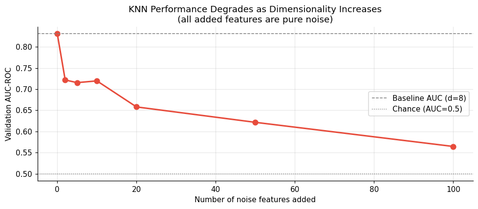
KNN AUC as irrelevant noise features are added:
 Noise features    Total d    Val AUC  Note
───────────────────────────────────────────────────────
              0          8      0.831 ← baseline
              2         10      0.722
              5         13      0.715
             10         18      0.720
             20         28      0.658
             50         58      0.622
            100        108      0.565 ← collapses
🤔 Reflection 4.1 — Dimensionality in Healthcare#
The max/min distance ratio collapses toward 1 as \(d\) grows. At \(d=100\), the ratio is close to 1, meaning all distances are nearly identical. What does this imply about the \(k\) nearest neighbors of a query point — are they meaningfully “similar” patients? How would you empirically test whether “nearest” means anything in a given dataset?
The noise feature experiment shows a smooth AUC decline as irrelevant features are added. Contrast this with logistic regression and decision trees: if you add 50 random noise features, would those models degrade as severely? Explain the mechanism that protects (or doesn’t protect) each model.
Dimensionality reduction (PCA, UMAP) is often applied before KNN in high-dimensional settings. What is the risk of applying PCA in a clinical prediction context? (Hint: think about what the principal components represent clinically — can you explain PC1 to a clinician? Does this matter if the model is just used for triage?)
A clinical researcher wants to use KNN on EHR data with 500 features. She argues that KNN is more interpretable than logistic regression because “this patient is similar to these 7 historical patients” is a natural explanation for a clinician. Do you agree with the interpretability claim? What are two fundamental problems with the 500-feature nearest-neighbor story from a clinical trust perspective?
Defining “similar” clinically: Suppose two patients have identical lab values but one is 30 and one is 70. Should they be considered “similar”? Identical diagnoses but different demographics? How would you incorporate clinical knowledge about which features should matter most into a KNN-style similarity metric — and is there an ML method that learns this automatically?
✅ Solution — Reflection 4.1#
1. At \(d=100\) with max/min ratio ≈ 1.1, the nearest neighbor is only ~10% closer than the farthest point. The \(k\) “nearest” neighbors are not meaningfully more similar to the query than any other training points. Empirically, you could test this by comparing the AUC of KNN to a model that predicts using \(k\) random training points instead of the \(k\) nearest — if both perform similarly, “nearest” is meaningless.
2. Logistic regression would not degrade as severely with 50 noise features. Its regularization (L2) would shrink the coefficients on noise features toward zero, effectively ignoring them. Decision trees also resist noise features — splits on noise features yield no information gain, so the tree won’t use them. KNN has no such protection: noise features contribute equally to the distance computation, diluting the signal.
3. PCA risk: the principal components are linear combinations of all features with no clinical meaning. PC1 might be “40% radius + 30% texture + 20% smoothness + …” which is uninterpretable. If the model is used only for triage (no explanation needed), this may be acceptable. But if a clinician asks “why was this patient flagged?”, you can’t point to a specific clinical feature. Additionally, PCA preserves variance, not discriminative information — the highest-variance direction may not separate classes well.
4. Two fundamental problems with 500-feature KNN: (a) Curse of dimensionality — at 500 dimensions, all distances are nearly equal, so the “7 most similar patients” are essentially random selections from the training set, not truly similar patients. (b) Defining similarity — with 500 features, two patients might be “nearest neighbors” because they share irrelevant features (same lab values for unrelated tests), not because they’re clinically similar in ways that matter for the outcome.
5. Age is a crucial example: a 30-year-old and 70-year-old with identical lab values should not be considered similar for most clinical predictions, because the baseline biology, treatment response, and prognosis differ enormously. Incorporating clinical knowledge requires weighting features by their clinical relevance in the distance metric. Metric learning methods (e.g., LMNN) can learn these weights automatically from labeled data, essentially learning “what does similarity mean for this prediction task?”
Part 5 — Evaluation, Calibration, and Comparison to Prior Models#
We now evaluate our best KNN model fully, and place it in context alongside logistic regression and the tree-based models from earlier labs. In clinical ML, no model exists in isolation — the question is always “compared to what, for what purpose?”
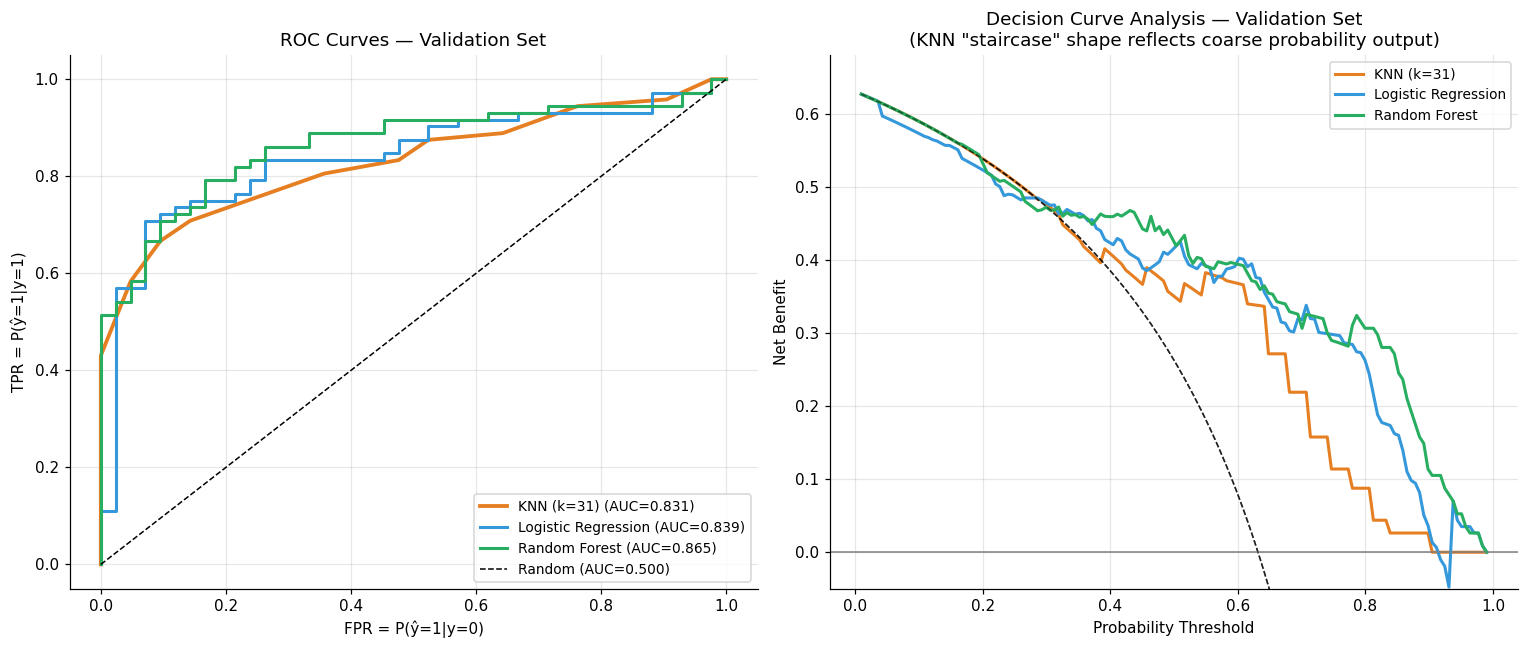
One important limitation to keep in mind: KNN’s coarse probability outputs (only \(k+1\) distinct values) mean that the decision curve analysis will show a “staircase” shape rather than a smooth curve. This is not a quirk of the data — it is a direct consequence of the probability discretization we examined in Part 3.
# Fit best KNN on training set; compare on validation set alongside prior models
from sklearn.linear_model import LogisticRegression
from sklearn.ensemble import RandomForestClassifier

best_knn = KNeighborsClassifier(n_neighbors=best_k)
best_knn.fit(X_train, y_train)

lr = LogisticRegression(C=1.0, max_iter=1000, random_state=42)
lr.fit(X_train, y_train)

rf = RandomForestClassifier(n_estimators=200, max_features='sqrt',
                             min_samples_leaf=3, random_state=42, n_jobs=-1)
rf.fit(X_train, y_train)

models = {
    f'KNN (k={best_k})':    best_knn,
    'Logistic Regression':  lr,
    'Random Forest':         rf,
}
colors = {'KNN (k=%d)' % best_k: '#e67e22',
          'Logistic Regression': '#3498db',
          'Random Forest':        '#27ae60'}

print("=== VALIDATION SET METRICS ===\n")
for name, model in models.items():
    preds = model.predict(X_val)
    probs = model.predict_proba(X_val)[:,1]
    print_metrics(y_val, preds, probs, label=name)
=== VALIDATION SET METRICS ===

───────────────────────────────────────────────────────
  KNN (k=31)
───────────────────────────────────────────────────────
  Sensitivity  P(ŷ=1|y=1)  = 60/72 = 0.833
  Specificity  P(ŷ=0|y=0)  = 22/42 = 0.524
  PPV          P(y=1|ŷ=1)  = 60/80 = 0.750
  NPV          P(y=0|ŷ=0)  = 22/34 = 0.647
  Prevalence               = 0.632
  AUC-ROC                  = 0.831

───────────────────────────────────────────────────────
  Logistic Regression
───────────────────────────────────────────────────────
  Sensitivity  P(ŷ=1|y=1)  = 60/72 = 0.833
  Specificity  P(ŷ=0|y=0)  = 29/42 = 0.690
  PPV          P(y=1|ŷ=1)  = 60/73 = 0.822
  NPV          P(y=0|ŷ=0)  = 29/41 = 0.707
  Prevalence               = 0.632
  AUC-ROC                  = 0.839

───────────────────────────────────────────────────────
  Random Forest
───────────────────────────────────────────────────────
  Sensitivity  P(ŷ=1|y=1)  = 57/72 = 0.792
  Specificity  P(ŷ=0|y=0)  = 33/42 = 0.786
  PPV          P(y=1|ŷ=1)  = 57/66 = 0.864
  NPV          P(y=0|ŷ=0)  = 33/48 = 0.688
  Prevalence               = 0.632
  AUC-ROC                  = 0.865
# ROC + DCA comparison on validation set
fig, axes = plt.subplots(1, 2, figsize=(14, 6))

for name, model in models.items():
    probs = model.predict_proba(X_val)[:,1]
    fpr, tpr, _ = roc_curve(y_val, probs)
    val_auc = auc(fpr, tpr)
    c = colors[name]
    lw = 2.5 if 'KNN' in name else 2.0
    axes[0].plot(fpr, tpr, lw=lw, color=c, label=f'{name} (AUC={val_auc:.3f})')
    nb = decision_curve(y_val, probs, label=name, ax=axes[1], color=c)

axes[0].plot([0,1],[0,1],'k--', lw=1, label='Random (AUC=0.500)')
axes[0].set_xlabel('FPR = P(ŷ=1|y=0)'); axes[0].set_ylabel('TPR = P(ŷ=1|y=1)')
axes[0].set_title('ROC Curves — Validation Set'); axes[0].legend(fontsize=9)
axes[0].grid(True, alpha=0.3)

axes[1].set_title('Decision Curve Analysis — Validation Set\n'
                  '(KNN "staircase" shape reflects coarse probability output)')
axes[1].legend(fontsize=9); axes[1].grid(True, alpha=0.3)

plt.tight_layout(); plt.show()
# Final: retrain on train+val, evaluate on test set
print("=== FINAL TEST SET EVALUATION ===")
print("(Models retrained on train+val, evaluated once on held-out test)\n")

X_tv = np.vstack([X_train, X_val])
y_tv = np.concatenate([y_train, y_val])

final_models = {
    f'KNN (k={best_k})':   KNeighborsClassifier(n_neighbors=best_k),
    'Logistic Regression': LogisticRegression(C=1.0, max_iter=1000, random_state=42),
    'Random Forest':        RandomForestClassifier(n_estimators=200, max_features='sqrt',
                                                    min_samples_leaf=3, random_state=42, n_jobs=-1),
}

test_aucs = {}
for name, model in final_models.items():
    model.fit(X_tv, y_tv)
    preds = model.predict(X_test)
    probs = model.predict_proba(X_test)[:,1]
    print_metrics(y_test, preds, probs, label=name)
    test_aucs[name] = roc_auc_score(y_test, probs)

# Summary bar chart
fig, ax = plt.subplots(figsize=(8, 4))
names = list(test_aucs.keys())
aucs_list = list(test_aucs.values())
bar_colors = [colors[n] for n in names]
bars = ax.bar(names, aucs_list, color=bar_colors, edgecolor='white', linewidth=1.5)
for bar, val in zip(bars, aucs_list):
    ax.text(bar.get_x()+bar.get_width()/2, bar.get_height()+0.003,
            f'{val:.3f}', ha='center', fontsize=12, fontweight='bold')
ax.set_ylabel('Test AUC-ROC'); ax.set_ylim(0.6, 1.0)
ax.set_title('Test Set AUC — Model Comparison\n(restricted feature set, n_train=120)')
ax.grid(True, alpha=0.3, axis='y')
plt.tight_layout(); plt.show()
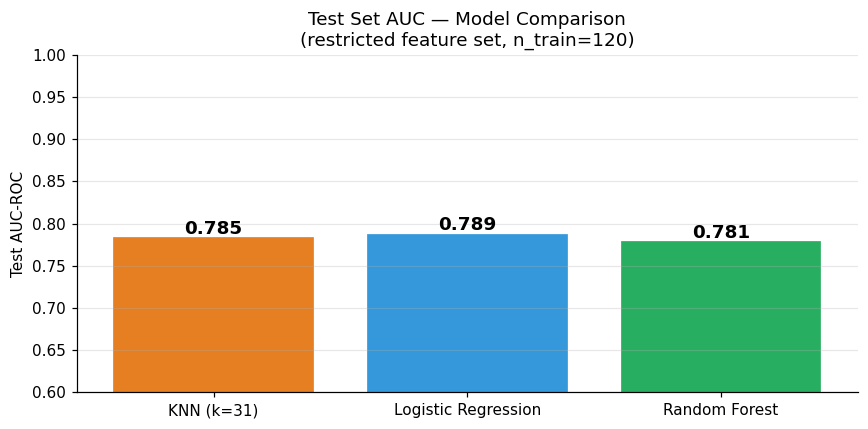
=== FINAL TEST SET EVALUATION ===
(Models retrained on train+val, evaluated once on held-out test)

───────────────────────────────────────────────────────
  KNN (k=31)
───────────────────────────────────────────────────────
  Sensitivity  P(ŷ=1|y=1)  = 54/71 = 0.761
  Specificity  P(ŷ=0|y=0)  = 26/43 = 0.605
  PPV          P(y=1|ŷ=1)  = 54/71 = 0.761
  NPV          P(y=0|ŷ=0)  = 26/43 = 0.605
  Prevalence               = 0.623
  AUC-ROC                  = 0.785

───────────────────────────────────────────────────────
  Logistic Regression
───────────────────────────────────────────────────────
  Sensitivity  P(ŷ=1|y=1)  = 62/71 = 0.873
  Specificity  P(ŷ=0|y=0)  = 26/43 = 0.605
  PPV          P(y=1|ŷ=1)  = 62/79 = 0.785
  NPV          P(y=0|ŷ=0)  = 26/35 = 0.743
  Prevalence               = 0.623
  AUC-ROC                  = 0.789
───────────────────────────────────────────────────────
  Random Forest
───────────────────────────────────────────────────────
  Sensitivity  P(ŷ=1|y=1)  = 60/71 = 0.845
  Specificity  P(ŷ=0|y=0)  = 23/43 = 0.535
  PPV          P(y=1|ŷ=1)  = 60/80 = 0.750
  NPV          P(y=0|ŷ=0)  = 23/34 = 0.676
  Prevalence               = 0.623
  AUC-ROC                  = 0.781
🤔 Reflection 5.1 — Evaluating KNN in Clinical Context#
Look at the DCA curves. KNN’s curve has a visibly staircase shape, while logistic regression and random forest are smooth. Explain why this happens mechanically. At a threshold of \(t = 0.14\) (approximately \(1/7\) for \(k=7\)), what does the model do for all patients with predicted probability between 0.14 and 0.28?
If the test AUC ordering is RF > LR > KNN, does that mean KNN should never be used? Describe a realistic clinical scenario where you would prefer KNN over a random forest, despite lower AUC. (Hint: think about the “similar patients” explanation and what clinicians find convincing when overriding a model.)
In contrast, describe a setting in which, even with a high AUC, a KNN may not be a good choice? What additional challenges does a KNN pose? What assumptions are “hidden” in a KNN that may be more visible in, for example, a logistic regression model? If you were to try to use a KNN in practice, what “non-technical” barriers might you encounter?
The models were evaluated on the same held-out test set. Suppose KNN wins on AUC but loses on sensitivity (missing more malignant cases). In the breast cancer screening context, which failure mode is more costly? How should this affect model selection — and is AUC even the right primary metric?
We used
predict_probafrom sklearn’s KNN, which uses uniform voting among neighbors. Sklearn also supportsweights='distance'(closer neighbors vote more strongly). Hypothesize whether distance-weighting would increase or decrease AUC here, and then test it in code.
✅ Solution — Reflection 5.1#
1. The staircase shape occurs because KNN probabilities can only take \(k+1\) values. As the decision threshold sweeps continuously from 0 to 1, the model’s predictions only change at the discrete probability values \(\{0, 1/k, 2/k, ...\}\). Between \(t=0.14\) and \(t=0.28\) (for \(k=7\)), the model treats all patients with predicted probability 1/7 identically — they are all either flagged or not flagged, with no gradation.
2. No — an AUC ranking (RF > LR > KNN) does not mean KNN should never be used. You might still prefer KNN when the decision workflow depends on a case-based, “similar patients” justification more than marginal gains in discriminative performance. For example: in an ED chest-pain triage tool used as decision support (not automation), clinicians often want to override the model for atypical or borderline presentations. A KNN system can say: “Here are the 7 most similar prior patients (age, troponin trend, ECG features, risk factors); 6/7 were ruled-in within 12 hours.” That auditable neighbor set gives clinicians something they can sanity-check (are these patients actually comparable?) and explain to others. Even with lower AUC, KNN can be more persuasive and safer in practice because it turns a prediction into a reviewable precedent rather than an opaque score.
3. Even with high AUC, KNN may be a poor choice in settings where the notion of “similarity” is unstable or clinically misleading, or where deployment requires robustness across sites. For example: sepsis prediction across multiple hospitals with different lab ordering patterns, units, and documentation habits. KNN can look great on held-out test data from one site, but fail when the feature distribution shifts (missingness patterns, measurement timing, coding differences). The extra challenges are: (i) KNN is extremely sensitive to feature scaling, missing data handling, and distance choice; (ii) its behavior can be dominated by spurious correlations or dense regions of the training set; (iii) it tends to degrade under dataset shift because “nearest neighbors” may stop being clinically comparable.
Hidden assumptions in KNN that are more explicit in LR include: local smoothness (“patients close in feature space have similar risk”), a particular metric defines clinical similarity, and the training set is a faithful reference population for future patients. Logistic regression makes assumptions more visible (e.g., linearity in the log-odds, which covariates matter, sign/direction of effects), which is often easier to critique and validate clinically.
Non-technical barriers: clinicians may distrust a tool if the “neighbors” are not explainable in clinical terms (e.g., similarity driven by billing codes or missingness), privacy/IRB constraints may limit showing patient-level exemplars, and governance teams may object to a system whose predictions implicitly rely on storing and retrieving individual historical cases (“are we making decisions by analogy to specific past patients?”).
4. In breast cancer screening, missing a malignant case (false negative) is far more costly than an unnecessary follow-up (false positive). If KNN has lower sensitivity, it is the worse model for this specific application, even with higher AUC. AUC is not the right primary metric here — sensitivity at a clinically relevant specificity (or net benefit at the relevant threshold) is more appropriate.
5. Distance-weighting (weights='distance') gives closer neighbors more influence, which should help when the \(k\) nearest neighbors include some that are much closer than others. With our small, low-dimensional dataset, it would likely produce a modest AUC improvement because it reduces the influence of “borderline” neighbors. You can test with: KNeighborsClassifier(n_neighbors=best_k, weights='distance').
🧠 Final Reflection — KNN in the ML Landscape#
Before moving to the next lab, synthesize what you’ve learned:
The inductive bias of KNN: Every ML model embeds assumptions about the world — its inductive bias. KNN’s is that nearby points in feature space have similar labels (Lipschitz smoothness). Write one sentence each explaining the inductive bias of: (a) logistic regression, (b) decision trees, (c) random forests. Which assumption is most likely to hold in a clinical dataset with noisy, heterogeneous EHR features?
The “no free lunch” theorem states that no algorithm is universally better than any other across all possible datasets. From our experiments, what properties of a dataset would favor KNN over logistic regression? What properties would favor logistic regression over KNN?
Memory-based vs. parametric: KNN is non-parametric — it makes no assumptions about the functional form of the decision boundary, and its complexity grows with \(n_{\text{train}}\). Logistic regression is parametric — it compresses the training data into a fixed number of parameters (\(d+1\)). In a federated healthcare setting where you cannot share patient records across hospitals, which type of model is easier to aggregate? Why?
When would you deploy KNN in production? Given what you know about computational cost, calibration, dimensionality sensitivity, and interpretability, sketch the conditions (dataset size, number of features, explanation requirements, latency budget) under which KNN would be your first choice for a clinical prediction task.
✅ Solution — Final Reflection#
1. Inductive biases: (a) Logistic regression: the log-odds of the outcome is a linear function of features — the decision boundary is a hyperplane. (b) Decision trees: the decision boundary is axis-aligned and hierarchical — the data can be partitioned by sequential feature thresholds. (c) Random forests: same as decision trees, but the true function is well-approximated by averaging many slightly different axis-aligned partitions. For noisy, heterogeneous EHR data, the random forest assumption is arguably most robust — it doesn’t require linearity and can adapt to complex interactions, while averaging reduces sensitivity to noise.
2. KNN is favored over logistic regression when: the decision boundary is highly non-linear, the number of features is small (< ~20), and data density is high (many samples per feature dimension). Logistic regression is favored when: features are high-dimensional (KNN suffers from curse of dimensionality), the relationship is approximately linear, the dataset is small (LR has fewer effective parameters), or probability calibration is critical.
3. In a federated setting where patient records cannot be shared, parametric models (logistic regression) are much easier to aggregate — you can average model weights across hospitals (federated averaging). KNN requires access to the raw data for prediction, which is incompatible with privacy constraints. You would need to either share the entire training set (violating privacy) or use approximate methods (which degrade performance).
4. KNN is a first choice when: (a) \(n_{\text{train}} < 10,000\) and \(d < 20\), (b) the “similar patients” explanation is specifically needed for clinical adoption, (c) the system must incorporate new cases without retraining, (d) latency requirements are relaxed (~100ms per query is acceptable), and (e) the features have been carefully selected to be clinically meaningful (so distance is interpretable). Outside these conditions, tree-based ensembles or logistic regression are usually better choices.