🔬 Lab 9: Probabilistic Regression

BINF 4002 – Machine Learning for Health

Lab 7 built regression models that output a single point estimate: “this tumor is predicted to be 15 mm.” But a clinician would immediately ask: “How sure are you?” A prediction of 15 mm with a 90% interval of [14, 16] means something very different from 15 mm with an interval of [5, 25].

This lab moves from point predictions to distributional predictions — models that output not just a best guess, but a full probability distribution over possible values. This is one of the most practically important upgrades in clinical ML, because clinical decisions almost always depend on the uncertainty around a prediction, not just the prediction itself.

We reuse the same dataset as Lab 7 (predicting mean radius from other features) so you can directly see how the same prediction problem is enriched by uncertainty.

Learning Objectives

1. Understand why point predictions are insufficient for clinical decision-making

2. Implement Gaussian negative log-likelihood (NLL) loss with heteroscedastic variance

3. Compare quantile regression to parametric distributional approaches

4. Evaluate calibration of probabilistic predictions (coverage, sharpness)

Set-up

Upload data

⚠️ First, you need to upload the pre-processed data from lab0. If you have issues with running the first lab, you can also download the data here.

Once you have downloaded the data locally and started the runtime for this notebook, upload the file to this notebook via the “Files” menu.

import os

pkl_path = 'processed_data.pkl'
if os.path.exists(pkl_path):
    print("✅ Data File Found!")
else:
    raise FileNotFoundError(
        "processed_data.pkl not found! "
        "Make sure you have run Lab 0 (lab0_preprocessing.ipynb) in full and "
        "downloaded the output (or used the link above), and uploaded it here."
    )

✅ Data File Found!

Imports and Data Setup (Same as Lab 7)

import numpy as np
import pandas as pd
import matplotlib.pyplot as plt
import matplotlib.gridspec as gridspec
import seaborn as sns
import pickle, warnings
from scipy import stats
warnings.filterwarnings('ignore')

plt.rcParams['figure.dpi'] = 110
plt.rcParams['axes.spines.top'] = False
plt.rcParams['axes.spines.right'] = False
sns.set_palette("Set2")

# ── Load data (identical to Lab 7 setup) ─────────────────────────────────────
with open('processed_data.pkl', 'rb') as f:
    d = pickle.load(f)

X_train_full = d['X_train']
X_val_full   = d['X_val']
X_test_full  = d['X_test']
feature_names_full = d['feature_names']
scaler = d['scaler']

# Target: mean radius in original mm units
target_idx = feature_names_full.index('mean radius')
target_mean  = scaler.mean_[target_idx]
target_scale = scaler.scale_[target_idx]

def to_original(z):
    return z * target_scale + target_mean

y_train = to_original(X_train_full[:, target_idx])
y_val   = to_original(X_val_full[:, target_idx])
y_test  = to_original(X_test_full[:, target_idx])

# Input features: drop radius/perimeter/area, add diagnosis label
drop_names = ['mean radius', 'mean perimeter', 'mean area']
drop_idx = [feature_names_full.index(n) for n in drop_names]
keep_idx = [i for i in range(len(feature_names_full)) if i not in drop_idx]

X_train = np.column_stack([X_train_full[:, keep_idx], d['y_train']])
X_val   = np.column_stack([X_val_full[:, keep_idx],   d['y_val']])
X_test  = np.column_stack([X_test_full[:, keep_idx],  d['y_test']])
feature_names = [feature_names_full[i] for i in keep_idx] + ['diagnosis (0=M, 1=B)']

print(f"Data: {X_train.shape[0]} train, {X_val.shape[0]} val, {X_test.shape[0]} test")
print(f"Features: {X_train.shape[1]}, Target: mean radius (mm)")
print(f"Target range: [{y_train.min():.1f}, {y_train.max():.1f}] mm")

Data: 341 train, 114 val, 114 test
Features: 28, Target: mean radius (mm)
Target range: [7.0, 25.2] mm

---

Part 1 — Motivation: Why Uncertainty Matters

Lab 7 produced point predictions. Let’s start by showing why that’s not enough.

# ── Train a point-estimate model (same as Lab 7) ─────────────────────────────
from sklearn.ensemble import GradientBoostingRegressor

gbr_point = GradientBoostingRegressor(n_estimators=200, max_depth=3, learning_rate=0.1,
                                       random_state=42)
gbr_point.fit(X_train, y_train)
yhat_val = gbr_point.predict(X_val)
residuals_val = y_val - yhat_val

print(f"Point model — Val RMSE: {np.sqrt(np.mean(residuals_val**2)):.2f} mm, "
      f"MAE: {np.mean(np.abs(residuals_val)):.2f} mm")

Point model — Val RMSE: 0.71 mm, MAE: 0.45 mm

# ── Find two patients with similar predictions but very different errors ──────
# Look for patients predicted to be ~14 mm
target_pred = np.median(yhat_val)
near_mask = np.abs(yhat_val - target_pred) < 0.5
near_idx = np.where(near_mask)[0]

if len(near_idx) >= 2:
    near_errors = np.abs(residuals_val[near_idx])
    sorted_by_error = near_idx[np.argsort(near_errors)]
    patient_good = sorted_by_error[0]     # small error
    patient_bad  = sorted_by_error[-1]    # large error
else:
    sorted_by_error = np.argsort(np.abs(residuals_val))
    patient_good = sorted_by_error[0]
    patient_bad  = sorted_by_error[-1]

fig, axes = plt.subplots(1, 2, figsize=(13, 4.5))

# Scatter of all predictions with these two highlighted
ax = axes[0]
ax.scatter(yhat_val, y_val, alpha=0.3, s=25, color='gray', edgecolors='white', linewidth=0.3)
ax.scatter(yhat_val[patient_good], y_val[patient_good], s=120, color=sns.color_palette('Set2')[2],
           edgecolors='black', linewidth=1.5, zorder=5, label='Patient A (small error)')
ax.scatter(yhat_val[patient_bad], y_val[patient_bad], s=120, color=sns.color_palette('Set2')[1],
           edgecolors='black', linewidth=1.5, zorder=5, label='Patient B (large error)')
lims = [y_val.min() - 1, y_val.max() + 1]
ax.plot(lims, lims, 'r--', linewidth=1)
ax.set_xlabel('Predicted (mm)'); ax.set_ylabel('Actual (mm)')
ax.set_title('Point Predictions Can\'t Distinguish\nEasy vs. Hard Patients', fontweight='bold')
ax.legend(fontsize=9)

# Show the problem: same prediction, different truth
ax = axes[1]
x_pos = [0, 1]
preds = [yhat_val[patient_good], yhat_val[patient_bad]]
actuals = [y_val[patient_good], y_val[patient_bad]]
colors = [sns.color_palette('Set2')[2], sns.color_palette('Set2')[1]]

for i, (p, a, c, lbl) in enumerate(zip(preds, actuals, colors,
                                         ['Patient A', 'Patient B'])):
    ax.bar(i, p, width=0.4, color=c, alpha=0.5, label=f'{lbl} predicted')
    ax.scatter(i, a, s=100, color=c, edgecolors='black', zorder=5, marker='D')
    ax.plot([i, i], [p, a], color='black', linewidth=1.5, linestyle=':')
    ax.annotate(f'error = {a-p:+.1f}', (i + 0.15, (p+a)/2), fontsize=9)

ax.set_xticks([0, 1])
ax.set_xticklabels(['Patient A', 'Patient B'])
ax.set_ylabel('Radius (mm)')
ax.set_title('Same Prediction, Different Reality\n(bars = predicted, ◆ = actual)', fontweight='bold')

plt.tight_layout()
plt.show()

print(f"Patient A: predicted {yhat_val[patient_good]:.1f} mm, actual {y_val[patient_good]:.1f} mm "
      f"(error {residuals_val[patient_good]:+.1f})")
print(f"Patient B: predicted {yhat_val[patient_bad]:.1f} mm, actual {y_val[patient_bad]:.1f} mm "
      f"(error {residuals_val[patient_bad]:+.1f})")
print("\n→ The point prediction tells us NOTHING about which patient's prediction to trust.")
print("  A probabilistic model would give Patient A a narrow interval and Patient B a wide one.")

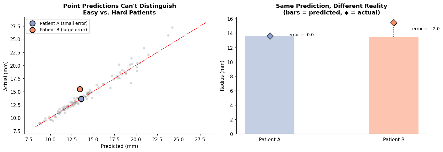
Patient A: predicted 13.6 mm, actual 13.6 mm (error -0.0)
Patient B: predicted 13.5 mm, actual 15.5 mm (error +2.0)

→ The point prediction tells us NOTHING about which patient's prediction to trust.
  A probabilistic model would give Patient A a narrow interval and Patient B a wide one.

🤔 Reflection 1.1 — When Uncertainty Changes the Decision

1. A model predicts tumor radius = 15 mm. Would a surgeon treat this differently if the 90% prediction interval is [14, 16] vs. [5, 25]? Think about surgical planning, margin determination, or treatment eligibility.

2. Name a clinical decision where the uncertainty around a prediction matters as much as (or more than) the prediction itself. (Examples: drug dosing near a toxicity threshold, cancer screening where false negatives are costly, surgical vs. conservative treatment where the risk-benefit balance is close.)

3. In Lab 7, we diagnosed heteroscedasticity — residuals were larger for larger tumors. A point model can’t capture this. A probabilistic model should predict wider intervals for larger tumors. Why is this clinically important?

---

Part 2 — Gaussian NLL: Predicting Mean and Variance

A standard regression model outputs a single value \(\hat{y} = f(\mathbf{x})\). A probabilistic regression model outputs a full distribution. The simplest approach assumes a Gaussian:

\[Y | \mathbf{x} \sim \mathcal{N}\big(\hat{\mu}(\mathbf{x}),\; \hat{\sigma}^2(\mathbf{x})\big)\]

The model has two outputs per patient:

• \(\hat{\mu}(\mathbf{x})\): the predicted mean (like Lab 7)

• \(\hat{\sigma}^2(\mathbf{x})\): the predicted variance (NEW — patient-specific uncertainty)

The Gaussian Negative Log-Likelihood (NLL) loss trains both heads jointly:

\[\mathcal{L} = \frac{1}{2n} \sum_{i=1}^{n} \left[ \frac{(y_i - \hat{\mu}_i)^2}{\hat{\sigma}_i^2} + \log \hat{\sigma}_i^2 \right]\]

This loss has two competing terms:

• \(\frac{(y - \hat{\mu})^2}{\hat{\sigma}^2}\): rewards predicting the correct mean, down-weighted when \(\hat{\sigma}^2\) is large

• \(\log \hat{\sigma}^2\): penalizes predicting large variance (prevents the model from cheating by making \(\hat{\sigma} \to \infty\))

def gaussian_nll_solution(y, mu_hat, sigma2_hat, eps=1e-8):
    """Gaussian Negative Log-Likelihood loss."""
    sigma2_safe = np.maximum(sigma2_hat, eps)
    squared_term = (y - mu_hat) ** 2 / sigma2_safe
    log_term = np.log(sigma2_safe)
    nll = (1 / (2 * len(y))) * np.sum(squared_term + log_term)
    return nll

# Verify
y_ck = np.array([10.0, 15.0, 20.0])
mu_ck = np.array([10.0, 15.0, 20.0])
sig2_ck = np.array([1.0, 1.0, 1.0])

print(f"Perfect mu, σ²=1:   NLL = {gaussian_nll_solution(y_ck, mu_ck, sig2_ck):.4f}  (≈ 0)")
print(f"Perfect mu, σ²=100: NLL = {gaussian_nll_solution(y_ck, mu_ck, np.array([100,100,100.])):.4f}  (≈ log(100)/2 = {np.log(100)/2:.2f})")

mu_bad = np.array([20.0, 5.0, 10.0])
print(f"Bad mu, σ²=1:       NLL = {gaussian_nll_solution(y_ck, mu_bad, sig2_ck):.4f}  (very high)")
print(f"Bad mu, σ²=100:     NLL = {gaussian_nll_solution(y_ck, mu_bad, np.array([100,100,100.])):.4f}  (lower — honest about uncertainty)")

Perfect mu, σ²=1:   NLL = 0.0000  (≈ 0)
Perfect mu, σ²=100: NLL = 2.3026  (≈ log(100)/2 = 2.30)
Bad mu, σ²=1:       NLL = 50.0000  (very high)
Bad mu, σ²=100:     NLL = 2.8026  (lower — honest about uncertainty)

# The key TODO lines in the training loop:
# mu_tr    = X_train @ w_mu + b_mu
# log_s_tr = X_train @ w_ls + b_ls
# d_mu     = (mu_tr - y_train) / sig2_tr
# d_log_s  = 0.5 * (1.0 - (y_train - mu_tr)**2 / sig2_tr)

# Here's a standalone solution:
def train_gaussian_nll_solution(X_tr, y_tr, X_vl, y_vl, lr_mu=0.001, lr_ls=0.0001, n_epochs=1500):
    np.random.seed(42)
    n, d_feat = X_tr.shape

    w_mu = np.random.randn(d_feat) * 0.01
    b_mu = y_tr.mean()
    w_ls = np.zeros(d_feat)
    b_ls = np.log(y_tr.var())

    train_nlls, val_nlls = [], []

    for epoch in range(n_epochs):
        mu_tr = X_tr @ w_mu + b_mu
        log_s_tr = X_tr @ w_ls + b_ls
        sig2_tr = np.exp(np.clip(log_s_tr, -10, 10))

        nll_tr = gaussian_nll_solution(y_tr, mu_tr, sig2_tr)

        d_mu = (mu_tr - y_tr) / sig2_tr
        d_log_s = 0.5 * (1.0 - (y_tr - mu_tr)**2 / sig2_tr)

        dw_mu = X_tr.T @ d_mu / n
        db_mu = d_mu.mean()
        dw_ls = X_tr.T @ d_log_s / n
        db_ls = d_log_s.mean()

        w_mu -= lr_mu * dw_mu;  b_mu -= lr_mu * db_mu
        w_ls -= lr_ls * dw_ls;  b_ls -= lr_ls * db_ls

        mu_vl = X_vl @ w_mu + b_mu
        sig2_vl = np.exp(np.clip(X_vl @ w_ls + b_ls, -10, 10))
        nll_vl = gaussian_nll_solution(y_vl, mu_vl, sig2_vl)

        train_nlls.append(nll_tr)
        val_nlls.append(nll_vl)

        if epoch % 300 == 0 or epoch == n_epochs - 1:
            print(f"Epoch {epoch:4d} | Train NLL: {nll_tr:.4f} | Val NLL: {nll_vl:.4f} | "
                  f"Mean σ(val): {np.sqrt(sig2_vl).mean():.2f}")

    return w_mu, b_mu, w_ls, b_ls, train_nlls, val_nlls

print("Solution function defined.")
print("Key insight: two separate 'heads' — one for mean (mu), one for log-variance (log_s).")
print("The exp() of log_s ensures variance is always positive.")

Solution function defined.
Key insight: two separate 'heads' — one for mean (mu), one for log-variance (log_s).
The exp() of log_s ensures variance is always positive.

# ── Plot NLL loss curves ─────────────────────────────────────────────────────
fig, ax = plt.subplots(figsize=(8, 4))
ax.plot(train_nlls, label='Train NLL', linewidth=2)
ax.plot(val_nlls, label='Validation NLL', linewidth=2, linestyle='--')
ax.set_xlabel('Epoch')
ax.set_ylabel('Gaussian NLL')
ax.set_title('Two-Headed Linear Model: Gaussian NLL Training', fontweight='bold')
ax.legend()
plt.tight_layout()
plt.show()

---------------------------------------------------------------------------
NameError                                 Traceback (most recent call last)
Cell In[7], line 3
      1 # ── Plot NLL loss curves ─────────────────────────────────────────────────────
      2 fig, ax = plt.subplots(figsize=(8, 4))
----> 3 ax.plot(train_nlls, label='Train NLL', linewidth=2)
      4 ax.plot(val_nlls, label='Validation NLL', linewidth=2, linestyle='--')
      5 ax.set_xlabel('Epoch')
      6 ax.set_ylabel('Gaussian NLL')

NameError: name 'train_nlls' is not defined

🤔 Reflection 2.1 — The Gaussian NLL Loss

1. Why do we predict \(\log \sigma^2\) instead of \(\sigma^2\) directly? (Hint: \(\exp(\cdot)\) maps \(\mathbb{R} \to \mathbb{R}^+\), so the model can’t accidentally predict a negative variance.)

2. What happens to the loss if the model predicts \(\hat{\sigma}^2 \to 0\) everywhere? The squared error term \(\frac{(y - \hat{\mu})^2}{\hat{\sigma}^2} \to \infty\) for any imperfect \(\hat{\mu}\). So the model is forced to be honest: it can only claim low uncertainty where it actually predicts accurately. Explain this tension.

3. If we set \(\hat{\sigma}^2\) to be a constant (same for all patients), the Gaussian NLL reduces to MSE (up to a constant). Verify this algebraically. This shows that MSE is a special case of Gaussian NLL — the homoscedastic case.

---

Part 3 — Quantile Regression

Gaussian NLL assumes the errors are normally distributed. Quantile regression makes no distributional assumptions. Instead of modeling \(P(Y | X)\) as a Gaussian, it directly estimates specific quantiles (e.g., the 10th, 50th, 90th percentiles) using the pinball loss:

\[\begin{split}L_q(y, \hat{y}) = \begin{cases} q \cdot (y - \hat{y}) & \text{if } y \geq \hat{y} \\ (1-q) \cdot (\hat{y} - y) & \text{if } y < \hat{y} \end{cases}\end{split}\]

Or equivalently: \(L_q(y, \hat{y}) = q \cdot \max(y - \hat{y}, 0) + (1-q) \cdot \max(\hat{y} - y, 0)\)

Intuition:

• \(q = 0.5\): pinball loss = MAE/2 → predicts the median

• \(q = 0.9\): under-prediction (actual above predicted) is penalized 9× more than over-prediction → model errs on the high side → predicts the 90th percentile

• \(q = 0.1\): over-prediction is penalized 9× more → predicts the 10th percentile

def pinball_loss_solution(y, y_hat, q):
    """Pinball (quantile) loss."""
    residual = y - y_hat
    loss = q * np.maximum(residual, 0) + (1 - q) * np.maximum(-residual, 0)
    return np.mean(loss)

# Verify
y_ck = np.array([10.0, 15.0, 20.0])
yhat_ck = np.array([12.0, 15.0, 18.0])

pb_50 = pinball_loss_solution(y_ck, yhat_ck, q=0.5)
mae_half = np.mean(np.abs(y_ck - yhat_ck)) / 2
print(f"q=0.5: {pb_50:.4f}, MAE/2: {mae_half:.4f}  (should match)")

pb_90 = pinball_loss_solution(y_ck, yhat_ck, q=0.9)
pb_10 = pinball_loss_solution(y_ck, yhat_ck, q=0.1)
print(f"q=0.9: {pb_90:.4f}  (under-predictions costly)")
print(f"q=0.1: {pb_10:.4f}  (over-predictions costly)")

q=0.5: 0.6667, MAE/2: 0.6667  (should match)
q=0.9: 0.6667  (under-predictions costly)
q=0.1: 0.6667  (over-predictions costly)

# ── Visualize the pinball loss for different quantiles ────────────────────────
errors = np.linspace(-5, 5, 200)   # y - y_hat

fig, ax = plt.subplots(figsize=(8, 4.5))
for q, color in zip([0.1, 0.25, 0.5, 0.75, 0.9],
                     sns.color_palette('viridis', 5)):
    loss_vals = q * np.maximum(errors, 0) + (1 - q) * np.maximum(-errors, 0)
    ax.plot(errors, loss_vals, color=color, linewidth=2, label=f'q={q}')

ax.set_xlabel('Residual ($y - \hat{y}$)')
ax.set_ylabel('Pinball Loss')
ax.set_title('Pinball Loss: Asymmetric Penalty for Different Quantiles', fontweight='bold')
ax.axvline(0, color='gray', linewidth=0.5, linestyle=':')
ax.legend()
plt.tight_layout()
plt.show()

print("q=0.9: steep left side → costly to predict TOO LOW (under the 90th %ile)")
print("q=0.1: steep right side → costly to predict TOO HIGH (over the 10th %ile)")

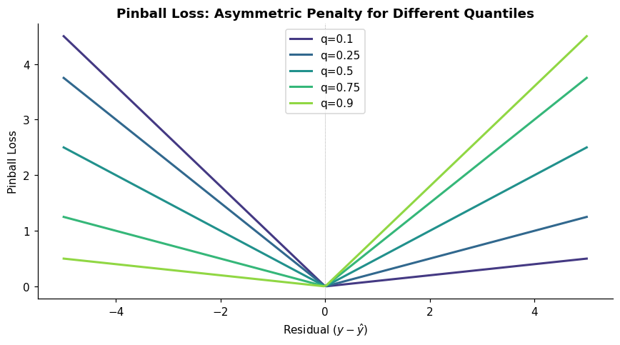
q=0.9: steep left side → costly to predict TOO LOW (under the 90th %ile)
q=0.1: steep right side → costly to predict TOO HIGH (over the 10th %ile)

# ── Fit quantile regressions ─────────────────────────────────────────────────
from sklearn.linear_model import QuantileRegressor

quantiles = [0.05, 0.10, 0.25, 0.50, 0.75, 0.90, 0.95]
qr_models = {}
qr_preds_val = {}

for q in quantiles:
    qr = QuantileRegressor(quantile=q, alpha=0.01, solver='highs')
    qr.fit(X_train, y_train)
    qr_models[q] = qr
    qr_preds_val[q] = qr.predict(X_val)
    print(f"q={q:.2f} — Val pinball loss: {pinball_loss(y_val, qr_preds_val[q], q):.4f}")

---------------------------------------------------------------------------
NameError                                 Traceback (most recent call last)
Cell In[10], line 13
      9     qr = QuantileRegressor(quantile=q, alpha=0.01, solver='highs')
     10     qr.fit(X_train, y_train)
     11     qr_models[q] = qr
     12     qr_preds_val[q] = qr.predict(X_val)
---> 13     print(f"q={q:.2f} — Val pinball loss: {pinball_loss(y_val, qr_preds_val[q], q):.4f}")

NameError: name 'pinball_loss' is not defined

# ── Visualize prediction intervals for individual patients ───────────────────
# Sort validation patients by predicted median for cleaner visualization
sort_idx = np.argsort(qr_preds_val[0.50])
n_show = min(40, len(y_val))
show_idx = sort_idx[np.linspace(0, len(sort_idx)-1, n_show, dtype=int)]

fig, ax = plt.subplots(figsize=(14, 5))

x_pos = np.arange(n_show)

# 90% interval (5th-95th percentile)
lo_90 = qr_preds_val[0.05][show_idx]
hi_90 = qr_preds_val[0.95][show_idx]
ax.fill_between(x_pos, lo_90, hi_90, alpha=0.2, color=sns.color_palette('Set2')[0],
                label='90% interval')

# 50% interval (25th-75th percentile)
lo_50 = qr_preds_val[0.25][show_idx]
hi_50 = qr_preds_val[0.75][show_idx]
ax.fill_between(x_pos, lo_50, hi_50, alpha=0.4, color=sns.color_palette('Set2')[0],
                label='50% interval')

# Median prediction
ax.plot(x_pos, qr_preds_val[0.50][show_idx], 'o-', color=sns.color_palette('Set2')[0],
        markersize=3, linewidth=1, label='Median prediction')

# True values
ax.scatter(x_pos, y_val[show_idx], color=sns.color_palette('Set2')[1], s=20,
           zorder=5, edgecolors='black', linewidth=0.5, label='True value')

ax.set_xlabel('Patient (sorted by predicted median)')
ax.set_ylabel('Mean Radius (mm)')
ax.set_title('Quantile Regression Prediction Intervals', fontweight='bold')
ax.legend(fontsize=9, loc='upper left')
plt.tight_layout()
plt.show()

print("Each patient gets a DIFFERENT interval width — wider where the model is less certain.")

---------------------------------------------------------------------------
KeyError                                  Traceback (most recent call last)
Cell In[11], line 3
      1 # ── Visualize prediction intervals for individual patients ───────────────────
      2 # Sort validation patients by predicted median for cleaner visualization
----> 3 sort_idx = np.argsort(qr_preds_val[0.50])
      4 n_show = min(40, len(y_val))
      5 show_idx = sort_idx[np.linspace(0, len(sort_idx)-1, n_show, dtype=int)]
      6 

KeyError: 0.5

🤔 Reflection 3.1 — Quantile vs. Gaussian

1. Quantile regression makes no distributional assumptions — it directly estimates percentiles. Gaussian NLL assumes normality. When might each be preferable? (Hint: for skewed targets, quantile regression can capture asymmetric intervals naturally, while the Gaussian model forces symmetric intervals around the mean.)

2. Quantile regression can produce crossing quantiles — e.g., the predicted 90th percentile for a patient might be below the predicted 10th percentile. Is this a bug or a fundamental limitation? How would you fix it?

3. Look at the prediction intervals above. Are they wider for some patients than others? What features might drive larger uncertainty?

---

Part 4 — Calibration of Probabilistic Predictions

A probabilistic model is only useful if its uncertainty estimates are calibrated: if the model says “there’s a 90% chance the true value is in [a, b]”, then ~90% of the time the true value should actually fall in that interval.

Two key concepts:

• Coverage: the fraction of true values inside the predicted interval (should match the nominal level)

• Sharpness: the average width of the interval (narrower is better, given correct coverage)

def empirical_coverage_solution(y_true, lower, upper):
    """Fraction of true values inside [lower, upper]."""
    inside = (y_true >= lower) & (y_true <= upper)
    return np.mean(inside)

# Verify
y_demo = np.array([1, 2, 3, 4, 5.0])
lo_demo = np.array([0.5, 1.5, 2.5, 3.5, 4.5])
hi_demo = np.array([1.5, 2.5, 3.5, 4.5, 5.5])
print(f"Coverage: {empirical_coverage_solution(y_demo, lo_demo, hi_demo):.1%}  (should be 100%)")

hi_narrow = np.array([1.5, 2.5, 3.5, 4.5, 4.9])  # last one misses
print(f"Coverage: {empirical_coverage_solution(y_demo, lo_demo, hi_narrow):.1%}  (should be 80%)")

Coverage: 100.0%  (should be 100%)
Coverage: 80.0%  (should be 80%)

# ── Calibration of Gaussian NLL model ────────────────────────────────────────
from scipy.stats import norm

# Get predictions from the trained Gaussian model
mu_val_gauss  = X_val @ w_mu + b_mu
sig2_val_gauss = np.exp(np.clip(X_val @ w_ls + b_ls, -10, 10))
sig_val_gauss  = np.sqrt(sig2_val_gauss)

# Build Gaussian intervals at different levels
print("Gaussian NLL Model — Calibration Check (Validation Set):")
print("─" * 65)
print(f"{'Interval':20s} {'Nominal':>10s} {'Observed':>10s} {'Width (mm)':>12s} {'Calibrated?':>12s}")
print("─" * 65)

for nominal in [0.50, 0.80, 0.90]:
    alpha = 1 - nominal
    z = norm.ppf(1 - alpha / 2)  # e.g., 1.645 for 90%
    lo_g = mu_val_gauss - z * sig_val_gauss
    hi_g = mu_val_gauss + z * sig_val_gauss
    cov = empirical_coverage(y_val, lo_g, hi_g)
    sharp = interval_sharpness(lo_g, hi_g)
    cal = '✅' if abs(cov - nominal) < 0.05 else '⚠️'
    print(f"{nominal:.0%} Gaussian:         {nominal:10.0%} {cov:10.1%} {sharp:12.2f} {cal:>12s}")

---------------------------------------------------------------------------
NameError                                 Traceback (most recent call last)
Cell In[13], line 5
      1 # ── Calibration of Gaussian NLL model ────────────────────────────────────────
      2 from scipy.stats import norm
      3 
      4 # Get predictions from the trained Gaussian model
----> 5 mu_val_gauss  = X_val @ w_mu + b_mu
      6 sig2_val_gauss = np.exp(np.clip(X_val @ w_ls + b_ls, -10, 10))
      7 sig_val_gauss  = np.sqrt(sig2_val_gauss)
      8 

NameError: name 'w_mu' is not defined

# ── Calibration curves ───────────────────────────────────────────────────────
nominal_levels = np.arange(0.10, 1.00, 0.05)

fig, axes = plt.subplots(1, 2, figsize=(13, 5))

# Quantile regression calibration
ax = axes[0]
qr_coverages = []
for level in nominal_levels:
    q_lo = (1 - level) / 2
    q_hi = 1 - q_lo
    # Need to fit/interpolate for quantiles we didn't fit
    # Use closest available quantiles
    if q_lo in qr_preds_val and q_hi in qr_preds_val:
        cov = empirical_coverage(y_val, qr_preds_val[q_lo], qr_preds_val[q_hi])
    else:
        cov = np.nan
    qr_coverages.append(cov)

# Gaussian calibration
gauss_coverages = []
for level in nominal_levels:
    z = norm.ppf(1 - (1 - level) / 2)
    lo_g = mu_val_gauss - z * sig_val_gauss
    hi_g = mu_val_gauss + z * sig_val_gauss
    gauss_coverages.append(empirical_coverage(y_val, lo_g, hi_g))

ax.plot([0, 1], [0, 1], 'k--', linewidth=1, label='Perfect calibration')
ax.plot(nominal_levels, gauss_coverages, 'o-', linewidth=2, markersize=4,
        label='Gaussian NLL', color=sns.color_palette('Set2')[0])
# Plot available QR points
valid_qr = [(n, c) for n, c in zip(nominal_levels, qr_coverages) if not np.isnan(c)]
if valid_qr:
    ax.plot([x[0] for x in valid_qr], [x[1] for x in valid_qr], 's-', linewidth=2,
            markersize=5, label='Quantile Regression', color=sns.color_palette('Set2')[1])

ax.set_xlabel('Nominal Coverage Level')
ax.set_ylabel('Observed Coverage')
ax.set_title('Probabilistic Calibration Curve', fontweight='bold')
ax.legend(fontsize=9)
ax.set_xlim(0, 1); ax.set_ylim(0, 1)
ax.set_aspect('equal')

# Sharpness comparison
ax = axes[1]
gauss_widths = []
for level in nominal_levels:
    z = norm.ppf(1 - (1 - level) / 2)
    gauss_widths.append(np.mean(2 * z * sig_val_gauss))

ax.plot(nominal_levels, gauss_widths, 'o-', linewidth=2, markersize=4,
        label='Gaussian NLL', color=sns.color_palette('Set2')[0])
ax.set_xlabel('Nominal Coverage Level')
ax.set_ylabel('Mean Interval Width (mm)')
ax.set_title('Sharpness: How Wide Are the Intervals?', fontweight='bold')
ax.legend(fontsize=9)

plt.tight_layout()
plt.show()

print("A well-calibrated model lies on the diagonal in the left plot.")
print("Above the diagonal = over-coverage (intervals too wide / conservative).")
print("Below the diagonal = under-coverage (intervals too narrow / overconfident).")

---------------------------------------------------------------------------
NameError                                 Traceback (most recent call last)
Cell In[14], line 24
     20 # Gaussian calibration
     21 gauss_coverages = []
     22 for level in nominal_levels:
     23     z = norm.ppf(1 - (1 - level) / 2)
---> 24     lo_g = mu_val_gauss - z * sig_val_gauss
     25     hi_g = mu_val_gauss + z * sig_val_gauss
     26     gauss_coverages.append(empirical_coverage(y_val, lo_g, hi_g))
     27 

NameError: name 'mu_val_gauss' is not defined

🤔 Reflection 4.1 — Coverage vs. Sharpness

1. Model A has 91% coverage at the 90% level (well-calibrated) but average interval width of 20 mm. Model B has 85% coverage (slightly under-calibrated) but width of 5 mm. Which is more clinically useful? How would you improve Model B?

2. A trivially “well-calibrated” model could predict \((-\infty, +\infty)\) for every patient — 100% coverage, but useless. This shows that coverage alone is insufficient. Why is sharpness (interval width) equally important?

3. Look at the calibration curve above. Is the Gaussian model over-confident or under-confident? What might cause miscalibration?

---

Part 5 — Heteroscedastic vs. Homoscedastic Models

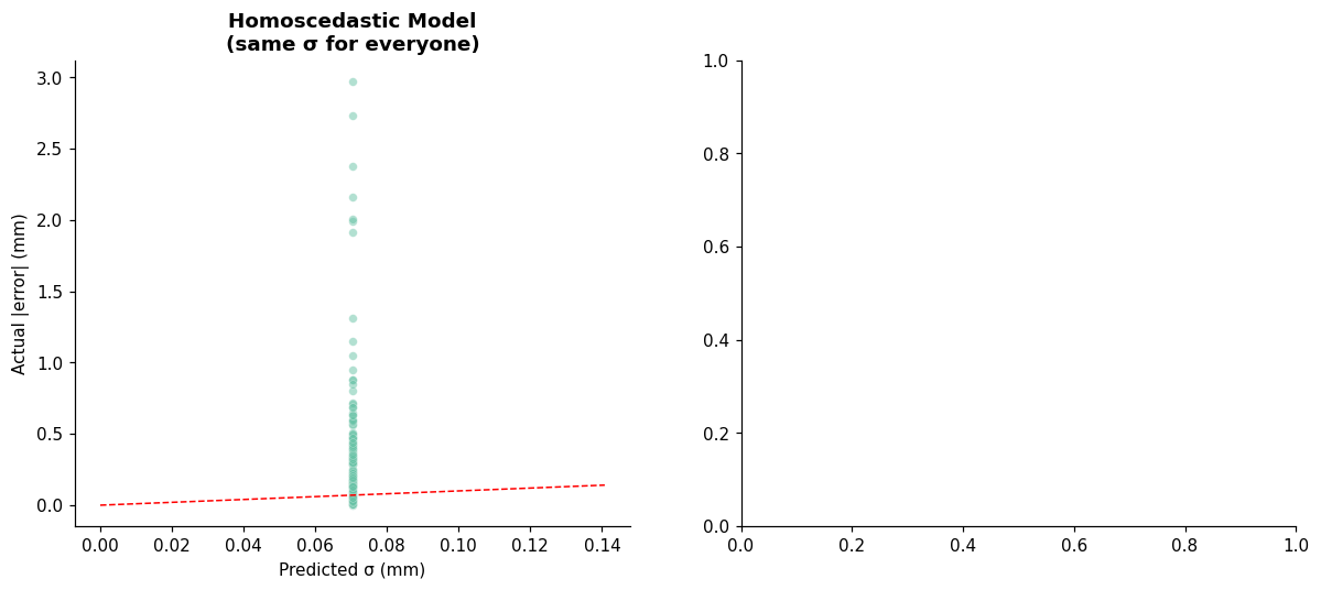
A homoscedastic model predicts the same uncertainty for all patients (one global \(\sigma^2\)). A heteroscedastic model predicts patient-specific uncertainty.

Lab 7 showed that residuals are larger for larger tumors (heteroscedasticity). A good probabilistic model should capture this — predicting wider intervals for harder cases.

# ── Build a homoscedastic baseline ───────────────────────────────────────────
# Use the point model from Part 1, plus a single global sigma estimated from
# training residuals.

yhat_train_point = gbr_point.predict(X_train)
residuals_train = y_train - yhat_train_point
sigma_global = residuals_train.std()

print(f"Homoscedastic model: global σ = {sigma_global:.2f} mm (same for all patients)")
print(f"Heteroscedastic model: σ ranges from {np.sqrt(sig2_val_gauss).min():.2f} "
      f"to {np.sqrt(sig2_val_gauss).max():.2f} mm")

Homoscedastic model: global σ = 0.07 mm (same for all patients)

---------------------------------------------------------------------------
NameError                                 Traceback (most recent call last)
Cell In[15], line 10
      6 residuals_train = y_train - yhat_train_point
      7 sigma_global = residuals_train.std()
      8 
      9 print(f"Homoscedastic model: global σ = {sigma_global:.2f} mm (same for all patients)")
---> 10 print(f"Heteroscedastic model: σ ranges from {np.sqrt(sig2_val_gauss).min():.2f} "
     11       f"to {np.sqrt(sig2_val_gauss).max():.2f} mm")

NameError: name 'sig2_val_gauss' is not defined

# ── Compare predicted uncertainty vs. actual error ────────────────────────────
fig, axes = plt.subplots(1, 2, figsize=(13, 5))

abs_errors_val = np.abs(y_val - yhat_val)

# Homoscedastic: everyone gets the same sigma
ax = axes[0]
ax.scatter(np.full_like(abs_errors_val, sigma_global), abs_errors_val,
           alpha=0.5, s=25, edgecolors='white', linewidth=0.3)
ax.set_xlabel('Predicted σ (mm)')
ax.set_ylabel('Actual |error| (mm)')
ax.set_title('Homoscedastic Model\n(same σ for everyone)', fontweight='bold')
ax.plot([0, sigma_global * 2], [0, sigma_global * 2], 'r--', linewidth=1)

# Heteroscedastic: patient-specific sigma
ax = axes[1]
ax.scatter(np.sqrt(sig2_val_gauss), abs_errors_val,
           alpha=0.5, s=25, edgecolors='white', linewidth=0.3)
ax.set_xlabel('Predicted σ (mm)')
ax.set_ylabel('Actual |error| (mm)')
ax.set_title('Heteroscedastic Model\n(patient-specific σ)', fontweight='bold')
lim = max(np.sqrt(sig2_val_gauss).max(), abs_errors_val.max()) + 1
ax.plot([0, lim], [0, lim], 'r--', linewidth=1, label='σ = |error|')
ax.legend(fontsize=9)

plt.tight_layout()
plt.show()

print("Ideally, points should scatter around the red line (predicted σ ≈ actual |error|).")
print("The heteroscedastic model should show a positive correlation (higher predicted σ → higher actual error).")

---------------------------------------------------------------------------
NameError                                 Traceback (most recent call last)
Cell In[16], line 17
     13 ax.plot([0, sigma_global * 2], [0, sigma_global * 2], 'r--', linewidth=1)
     14 
     15 # Heteroscedastic: patient-specific sigma
     16 ax = axes[1]
---> 17 ax.scatter(np.sqrt(sig2_val_gauss), abs_errors_val,
     18            alpha=0.5, s=25, edgecolors='white', linewidth=0.3)
     19 ax.set_xlabel('Predicted σ (mm)')
     20 ax.set_ylabel('Actual |error| (mm)')

NameError: name 'sig2_val_gauss' is not defined

# ── Stratify by predicted uncertainty tertiles ────────────────────────────────
sig_val = np.sqrt(sig2_val_gauss)
tertile_bounds = np.percentile(sig_val, [33.3, 66.7])
tertile_labels = ['Low σ', 'Medium σ', 'High σ']

tertile_groups = np.digitize(sig_val, tertile_bounds)

fig, axes = plt.subplots(1, 3, figsize=(15, 4))
colors = [sns.color_palette('Set2')[2], sns.color_palette('Set2')[0], sns.color_palette('Set2')[1]]

for group, label, color, ax in zip(range(3), tertile_labels, colors, axes):
    mask = tertile_groups == group
    errors_group = abs_errors_val[mask]
    sigma_group = sig_val[mask]

    ax.hist(errors_group, bins=15, color=color, edgecolor='white', alpha=0.8)
    ax.axvline(errors_group.mean(), color='black', linestyle='--',
               label=f'Mean |error| = {errors_group.mean():.2f} mm')
    ax.axvline(sigma_group.mean(), color='red', linestyle=':',
               label=f'Mean σ = {sigma_group.mean():.2f} mm')
    ax.set_xlabel('|Error| (mm)')
    ax.set_ylabel('Count')
    ax.set_title(f'{label} (n={mask.sum()})', fontweight='bold')
    ax.legend(fontsize=8)

plt.suptitle('Actual Errors Stratified by Predicted Uncertainty Tertiles',
             fontweight='bold', fontsize=12, y=1.03)
plt.tight_layout()
plt.show()

print("If the model is well-calibrated, patients in the 'High σ' group should have")
print("larger actual errors (wider spread) than those in the 'Low σ' group.")

# Quantify
for group, label in zip(range(3), tertile_labels):
    mask = tertile_groups == group
    print(f"  {label:10s}: mean |error| = {abs_errors_val[mask].mean():.2f} mm, "
          f"mean predicted σ = {sig_val[mask].mean():.2f} mm")

---------------------------------------------------------------------------
NameError                                 Traceback (most recent call last)
Cell In[17], line 2
      1 # ── Stratify by predicted uncertainty tertiles ────────────────────────────────
----> 2 sig_val = np.sqrt(sig2_val_gauss)
      3 tertile_bounds = np.percentile(sig_val, [33.3, 66.7])
      4 tertile_labels = ['Low σ', 'Medium σ', 'High σ']
      5 

NameError: name 'sig2_val_gauss' is not defined

🤔 Reflection 5.1 — Types of Uncertainty

1. The heteroscedastic model captures aleatoric uncertainty — inherent noise that can’t be reduced by collecting more data (e.g., measurement imprecision for large tumors). There’s also epistemic uncertainty — uncertainty due to lack of data (e.g., the model has seen few patients with rare feature combinations). Which type does the Gaussian NLL model capture? How could you estimate the other type?

2. Should a model used for clinical decision support distinguish between these two types? Consider: high aleatoric uncertainty means “we can’t know more even with better data.” High epistemic uncertainty means “we need more data like this patient.” These call for very different clinical responses.

3. Look at the tertile analysis. Does higher predicted uncertainty correspond to higher actual error? If so, the model’s uncertainty estimates are informative. If not, what might be going wrong?

---

Part 6 — Final Test Set Evaluation

Evaluate the probabilistic models on the held-out test set.

# ── Retrain the Gaussian NLL model on train + val ────────────────────────────
# For a proper final evaluation, we retrain on the combined data.
# We'll use the same hyperparameters (learning rates, epochs) selected on val.

X_tv = np.vstack([X_train, X_val])
y_tv = np.concatenate([y_train, y_val])

np.random.seed(42)
n_tv = X_tv.shape[0]
w_mu_f = np.random.randn(X_tv.shape[1]) * 0.01
b_mu_f = y_tv.mean()
w_ls_f = np.zeros(X_tv.shape[1])
b_ls_f = np.log(y_tv.var())

for epoch in range(n_epochs):
    mu_tv    = X_tv @ w_mu_f + b_mu_f
    log_s_tv = X_tv @ w_ls_f + b_ls_f
    sig2_tv  = np.exp(np.clip(log_s_tv, -10, 10))

    d_mu_f = (mu_tv - y_tv) / sig2_tv
    d_log_s_f = 0.5 * (1.0 - (y_tv - mu_tv)**2 / sig2_tv)

    w_mu_f -= lr_mu * (X_tv.T @ d_mu_f / n_tv)
    b_mu_f -= lr_mu * d_mu_f.mean()
    w_ls_f -= lr_ls * (X_tv.T @ d_log_s_f / n_tv)
    b_ls_f -= lr_ls * d_log_s_f.mean()

# Test predictions
mu_test  = X_test @ w_mu_f + b_mu_f
sig2_test = np.exp(np.clip(X_test @ w_ls_f + b_ls_f, -10, 10))
sig_test  = np.sqrt(sig2_test)

# Also retrain quantile models on train + val
qr_preds_test = {}
for q in quantiles:
    qr_f = QuantileRegressor(quantile=q, alpha=0.01, solver='highs')
    qr_f.fit(X_tv, y_tv)
    qr_preds_test[q] = qr_f.predict(X_test)

print("Models retrained on train+val.")

---------------------------------------------------------------------------
NameError                                 Traceback (most recent call last)
Cell In[18], line 15
     11 b_mu_f = y_tv.mean()
     12 w_ls_f = np.zeros(X_tv.shape[1])
     13 b_ls_f = np.log(y_tv.var())
     14 
---> 15 for epoch in range(n_epochs):
     16     mu_tv    = X_tv @ w_mu_f + b_mu_f
     17     log_s_tv = X_tv @ w_ls_f + b_ls_f
     18     sig2_tv  = np.exp(np.clip(log_s_tv, -10, 10))

NameError: name 'n_epochs' is not defined

# ── Final test evaluation ────────────────────────────────────────────────────
print("═" * 70)
print("  FINAL TEST SET EVALUATION — Probabilistic Models")
print("═" * 70)

# Point metrics
rmse_gauss = np.sqrt(np.mean((y_test - mu_test)**2))
mae_gauss  = np.mean(np.abs(y_test - mu_test))
rmse_qr    = np.sqrt(np.mean((y_test - qr_preds_test[0.50])**2))
mae_qr     = np.mean(np.abs(y_test - qr_preds_test[0.50]))

print(f"\n  Point prediction quality (median/mean):")
print(f"  {'Model':25s} {'RMSE (mm)':>10s} {'MAE (mm)':>10s}")
print(f"  " + "─" * 47)
print(f"  {'Gaussian NLL (mean)':25s} {rmse_gauss:10.2f} {mae_gauss:10.2f}")
print(f"  {'Quantile Reg (median)':25s} {rmse_qr:10.2f} {mae_qr:10.2f}")

# Calibration
print(f"\n  Calibration (coverage):")
print(f"  {'Interval':25s} {'Nominal':>10s} {'Gaussian':>10s} {'Quantile':>10s}")
print(f"  " + "─" * 57)

for name, q_lo, q_hi, nominal in intervals:
    # Gaussian
    z = norm.ppf(1 - (1 - nominal) / 2)
    cov_g = empirical_coverage(y_test, mu_test - z * sig_test, mu_test + z * sig_test)
    # Quantile
    if q_lo in qr_preds_test and q_hi in qr_preds_test:
        cov_q = empirical_coverage(y_test, qr_preds_test[q_lo], qr_preds_test[q_hi])
    else:
        cov_q = float('nan')
    print(f"  {name:25s} {nominal:10.0%} {cov_g:10.1%} {cov_q:10.1%}")

# Sharpness
sharp_g_90 = interval_sharpness(mu_test - 1.645 * sig_test, mu_test + 1.645 * sig_test)
sharp_q_90 = interval_sharpness(qr_preds_test[0.05], qr_preds_test[0.95])
print(f"\n  90% Interval Sharpness (mean width):")
print(f"  {'Gaussian NLL':25s} {sharp_g_90:.2f} mm")
print(f"  {'Quantile Regression':25s} {sharp_q_90:.2f} mm")

# NLL
nll_test = gaussian_nll(y_test, mu_test, sig2_test)
print(f"\n  Gaussian NLL on test set: {nll_test:.4f}")
print("═" * 70)

══════════════════════════════════════════════════════════════════════
  FINAL TEST SET EVALUATION — Probabilistic Models
══════════════════════════════════════════════════════════════════════

---------------------------------------------------------------------------
NameError                                 Traceback (most recent call last)
Cell In[19], line 7
      3 print("  FINAL TEST SET EVALUATION — Probabilistic Models")
      4 print("═" * 70)
      5 
      6 # Point metrics
----> 7 rmse_gauss = np.sqrt(np.mean((y_test - mu_test)**2))
      8 mae_gauss  = np.mean(np.abs(y_test - mu_test))
      9 rmse_qr    = np.sqrt(np.mean((y_test - qr_preds_test[0.50])**2))
     10 mae_qr     = np.mean(np.abs(y_test - qr_preds_test[0.50]))

NameError: name 'mu_test' is not defined

# ── Final visualization: prediction intervals on test set ────────────────────
sort_idx_test = np.argsort(mu_test)
n_show = min(40, len(y_test))
show_idx = sort_idx_test[np.linspace(0, len(sort_idx_test)-1, n_show, dtype=int)]

fig, ax = plt.subplots(figsize=(14, 5))
x_pos = np.arange(n_show)

# 90% Gaussian interval
z90 = 1.645
lo_g = (mu_test - z90 * sig_test)[show_idx]
hi_g = (mu_test + z90 * sig_test)[show_idx]
ax.fill_between(x_pos, lo_g, hi_g, alpha=0.25, color=sns.color_palette('Set2')[0],
                label='Gaussian 90% interval')
ax.plot(x_pos, mu_test[show_idx], 'o-', color=sns.color_palette('Set2')[0],
        markersize=3, linewidth=1, label='Gaussian mean')

# True values
ax.scatter(x_pos, y_test[show_idx], color=sns.color_palette('Set2')[1], s=25,
           zorder=5, edgecolors='black', linewidth=0.5, label='True value')

ax.set_xlabel('Patient (sorted by predicted mean)')
ax.set_ylabel('Mean Radius (mm)')
ax.set_title('Test Set — Gaussian NLL Prediction Intervals', fontweight='bold')
ax.legend(fontsize=9)
plt.tight_layout()
plt.show()

---------------------------------------------------------------------------
NameError                                 Traceback (most recent call last)
Cell In[20], line 2
      1 # ── Final visualization: prediction intervals on test set ────────────────────
----> 2 sort_idx_test = np.argsort(mu_test)
      3 n_show = min(40, len(y_test))
      4 show_idx = sort_idx_test[np.linspace(0, len(sort_idx_test)-1, n_show, dtype=int)]
      5 

NameError: name 'mu_test' is not defined

---

🤔 Final Reflection

A hospital deploys a model that predicts patient lab values (e.g., creatinine levels) with 95% prediction intervals. After a few months, clinicians notice that the intervals are always roughly the same width for every patient.

1. Type of uncertainty: What type of uncertainty is this model likely capturing — aleatoric or epistemic? What type is missing? (Hint: a homoscedastic model captures average noise but not patient-specific uncertainty.)

2. Clinical impact: A patient with stable kidney function and a patient with rapidly deteriorating kidney function both get the same-width interval around their creatinine prediction. Why is this dangerous? What clinical decisions might be affected?

3. How to fix it: How would you upgrade the model? Consider:

   • Switching from MSE to Gaussian NLL (to model heteroscedastic variance)

   • Using quantile regression (to capture asymmetric uncertainty)

   • Ensembling multiple models (to capture epistemic uncertainty) Which would you try first, and why?

4. Connection to Lab 7: Lab 7 diagnosed heteroscedasticity in the residuals but could only observe it post hoc. This lab equipped you to predict patient-specific uncertainty before seeing the outcome. Why is this shift — from retrospective diagnosis to prospective prediction — so valuable in clinical ML?