
Notebook 17: Exploring EHR Data with MIMIC-IV in MEDS Format#
BINF 4002 — Machine Learning for Health | Lecture 17 Companion
This notebook uses real clinical data — the MIMIC-IV demo dataset (100 ICU patients from Beth Israel Deaconess Medical Center), converted to the Medical Event Data Standard (MEDS) format.
We will:
Download and explore the MEDS data structure
Visualize patient timelines as event streams
Demonstrate Zipf’s law in medical code frequencies
Explore code ontology hierarchies and feature dimensionality
Show informative observation — sicker patients generate more data
Demonstrate Berkson’s Paradox using real diagnoses
Simulate an EHR → claims transformation and quantify information loss
Examine censoring and observation windows
Data source: MIMIC-IV demo in MEDS — openly available, no credentials required.
Key concept refresher: AUC = Area Under the ROC Curve (0.5 = random, 1.0 = perfect). Cross-validation = train/test on different folds for robust estimates.
# ── SETUP ──
# (pip install handled by the book's isolated env)

import numpy as np
import pandas as pd
import matplotlib.pyplot as plt
import matplotlib.patches as mpatches
import seaborn as sns
from scipy import stats
from scipy.stats import chi2_contingency
from sklearn.linear_model import LogisticRegression
from sklearn.metrics import roc_auc_score
from sklearn.model_selection import StratifiedKFold, cross_val_score
from collections import Counter
import warnings
warnings.filterwarnings("ignore")

sns.set_style("whitegrid")
PAL = sns.color_palette("colorblind")
plt.rcParams.update({"figure.figsize": (10, 5), "axes.titlesize": 13,
                      "axes.labelsize": 11, "font.size": 10})
np.random.seed(42)
print("Setup complete.")
/bin/bash: line 1: pip: command not found
Setup complete.
# ── DOWNLOAD MIMIC-IV DEMO IN MEDS FORMAT ──
import os, subprocess

MEDS_URL = "https://physionet.org/files/mimic-iv-demo-meds/0.0.1/"
DATA_DIR = "mimic-iv-demo-meds"

if not os.path.exists(DATA_DIR):
    print("Downloading MIMIC-IV demo in MEDS format (~1.5 MB)...")
    subprocess.run(["wget", "-r", "-N", "-c", "-np", "-nH", "--cut-dirs=1",
                    "-P", DATA_DIR, MEDS_URL],
                   check=True, capture_output=True)
    print("Download complete.")
else:
    print(f"Data already exists in {DATA_DIR}/")

# Show structure
for root, dirs, files in os.walk(DATA_DIR):
    level = root.replace(DATA_DIR, '').count(os.sep)
    indent = ' ' * 2 * level
    print(f'{indent}{os.path.basename(root)}/')
    for f in sorted(files):
        sz = os.path.getsize(os.path.join(root, f))
        print(f'{" " * 2 * (level+1)}{f} ({sz/1024:.1f} KB)')
Data already exists in mimic-iv-demo-meds/
mimic-iv-demo-meds/
  robots.txt (0.0 KB)
  mimic-iv-demo-meds/
    0.0.1/
      LICENSE.txt (25.2 KB)
      README.txt (1.4 KB)
      SHA256.txt (0.5 KB)
      SHA256SUMS.txt (0.7 KB)
      index.html (0.9 KB)
      data/
        index.html (0.6 KB)
        train/
          0.parquet (4747.0 KB)
          index.html (0.4 KB)
        tuning/
          0.parquet (414.1 KB)
          index.html (0.4 KB)
        held_out/
          0.parquet (265.1 KB)
          index.html (0.4 KB)
      metadata/
        codes.parquet (381.0 KB)
        dataset.json (0.2 KB)
        index.html (0.6 KB)
        subject_splits.parquet (1.3 KB)
# ── LOAD THE MEDS DATA ──
from pathlib import Path

data_dir = Path(DATA_DIR)
data_files = sorted(data_dir.rglob("data/**/*.parquet"))

dfs = [pd.read_parquet(f) for f in data_files]
for f, df in zip(data_files, dfs):
    print(f"  {f.name}: {len(df):,} rows")

meds = pd.concat(dfs, ignore_index=True)
print(f"\nTotal events: {len(meds):,} | Patients: {meds['subject_id'].nunique()}")
print(f"Columns: {list(meds.columns)}")
print(f"Code examples: {meds['code'].iloc[:5].tolist()}")
meds.head(8)
  0.parquet: 42,554 rows
  0.parquet: 803,992 rows
  0.parquet: 69,620 rows

Total events: 916,166 | Patients: 100
Columns: ['subject_id', 'time', 'code', 'numeric_value', 'insurance', 'language', 'marital_status', 'race', 'hadm_id', 'drg_severity', 'drg_mortality', 'emar_id', 'emar_seq', 'text_value', 'priority', 'route', 'frequency', 'doses_per_24_hrs', 'poe_id', 'icustay_id', 'order_id', 'link_order_id', 'unit', 'ordercategorydescription', 'statusdescription']
Code examples: ['GENDER//F', 'MEDS_BIRTH', 'Height (Inches)', 'Weight (Lbs)', 'BMI (kg/m2)']
| subject_id | time | code | numeric_value | insurance | language | marital_status | race | hadm_id | drg_severity | ... | route | frequency | doses_per_24_hrs | poe_id | icustay_id | order_id | link_order_id | unit | ordercategorydescription | statusdescription | |
|---|---|---|---|---|---|---|---|---|---|---|---|---|---|---|---|---|---|---|---|---|---|
| 0 | 10012853 | NaT | GENDER//F | NaN | NaN | NaN | NaN | NaN | NaN | NaN | ... | NaN | NaN | NaN | NaN | NaN | NaN | NaN | NaN | NaN | NaN |
| 1 | 10012853 | 2084-01-01 00:00:00 | MEDS_BIRTH | NaN | NaN | NaN | NaN | NaN | NaN | NaN | ... | NaN | NaN | NaN | NaN | NaN | NaN | NaN | NaN | NaN | NaN |
| 2 | 10012853 | 2175-04-05 00:00:00 | Height (Inches) | NaN | NaN | NaN | NaN | NaN | NaN | NaN | ... | NaN | NaN | NaN | NaN | NaN | NaN | NaN | NaN | NaN | NaN |
| 3 | 10012853 | 2175-04-05 00:00:00 | Weight (Lbs) | NaN | NaN | NaN | NaN | NaN | NaN | NaN | ... | NaN | NaN | NaN | NaN | NaN | NaN | NaN | NaN | NaN | NaN |
| 4 | 10012853 | 2175-04-05 00:00:00 | BMI (kg/m2) | NaN | NaN | NaN | NaN | NaN | NaN | NaN | ... | NaN | NaN | NaN | NaN | NaN | NaN | NaN | NaN | NaN | NaN |
| 5 | 10012853 | 2175-04-05 06:22:00 | ED_REGISTRATION | NaN | NaN | NaN | NaN | NaN | NaN | NaN | ... | NaN | NaN | NaN | NaN | NaN | NaN | NaN | NaN | NaN | NaN |
| 6 | 10012853 | 2175-04-05 06:22:00 | TRANSFER_TO//ED//Emergency Department | NaN | NaN | NaN | NaN | NaN | 26369609.0 | NaN | ... | NaN | NaN | NaN | NaN | NaN | NaN | NaN | NaN | NaN | NaN |
| 7 | 10012853 | 2175-04-05 06:30:00 | LAB//50955//UNK | NaN | NaN | NaN | NaN | NaN | NaN | NaN | ... | NaN | NaN | NaN | NaN | NaN | NaN | NaN | NaN | NaN | NaN |
8 rows × 25 columns
# ── PARSE MEDS CODE FORMAT & DOWNLOAD LOOKUP TABLES ──
# MEDS codes have format: TYPE//ONTOLOGY//CODE or TYPE//ITEMID//UNIT
# e.g. "DIAGNOSIS//ICD9CM//4019", "LAB//220045//bpm"

def parse_code(c):
    parts = str(c).split("//")
    return {
        "category": parts[0] if len(parts) >= 1 else "UNK",
        "ontology": parts[1] if len(parts) >= 2 else "",
        "detail": parts[2] if len(parts) >= 3 else "",
        "full": c
    }

parsed = meds["code"].apply(parse_code).apply(pd.Series)
meds["category"] = parsed["category"]
meds["ontology"] = parsed["ontology"]
meds["detail"] = parsed["detail"]

# Identify birth events (MEDS adds one at DOB, which inflates timelines)
meds["is_birth"] = meds["code"].str.contains("BIRTH|birth", case=False, na=False)

print("Event category distribution:")
print(meds["category"].value_counts().head(20).to_string())
print(f"\nBirth events: {meds['is_birth'].sum()} (one per patient)")

# ── Download MIMIC-IV demo lookup tables for human-readable names ──
import subprocess

DEMO_BASE = "https://physionet.org/files/mimic-iv-demo/2.2"
for table in ["hosp/d_icd_diagnoses.csv.gz", "hosp/d_icd_procedures.csv.gz", "icu/d_items.csv.gz"]:
    fname = table.split("/")[-1]
    if not os.path.exists(fname):
        subprocess.run(["wget", "-q", f"{DEMO_BASE}/{table}", "-O", fname], check=False)

# Build code-to-name lookup
code_names = {}

# ICD diagnoses
try:
    d_icd = pd.read_csv("d_icd_diagnoses.csv.gz")
    for _, row in d_icd.iterrows():
        code_names[str(row["icd_code"])] = row["long_title"]
    print(f"\nLoaded {len(d_icd)} ICD diagnosis names")
except Exception as e:
    print(f"Could not load d_icd_diagnoses: {e}")

# ICD procedures
try:
    d_proc = pd.read_csv("d_icd_procedures.csv.gz")
    for _, row in d_proc.iterrows():
        code_names[f"proc_{row['icd_code']}"] = row["long_title"]
    print(f"Loaded {len(d_proc)} ICD procedure names")
except Exception as e:
    print(f"Could not load d_icd_procedures: {e}")

# ICU items (labs, vitals, etc.)
try:
    d_items = pd.read_csv("d_items.csv.gz")
    for _, row in d_items.iterrows():
        code_names[str(row["itemid"])] = row["label"]
    print(f"Loaded {len(d_items)} ICU item names")
except Exception as e:
    print(f"Could not load d_items: {e}")

def resolve_code(meds_code):
    """Convert a MEDS code to a human-readable name."""
    parts = str(meds_code).split("//")
    category = parts[0] if len(parts) >= 1 else ""
    detail = parts[1] if len(parts) >= 2 else ""

    # For DIAGNOSIS codes, the ICD code is the last meaningful part
    if category == "DIAGNOSIS" and len(parts) >= 3:
        icd = parts[-1]
        if icd in code_names:
            return f"{icd}: {code_names[icd]}"

    # For LAB codes, the itemid is the second part
    if category == "LAB" and detail in code_names:
        return code_names[detail]

    # For procedures
    if category == "PROCEDURE" and len(parts) >= 3:
        icd = parts[-1]
        if f"proc_{icd}" in code_names:
            return f"{icd}: {code_names[f'proc_{icd}']}"

    # Fallback
    return str(meds_code).split("//")[-1] if "//" in str(meds_code) else str(meds_code)

# Test it
print("\nCode resolution examples:")
for c in meds["code"].value_counts().head(5).index:
    print(f"  {c} -> {resolve_code(c)}")
for c in meds[meds["category"]=="DIAGNOSIS"]["code"].value_counts().head(5).index:
    print(f"  {c} -> {resolve_code(c)}")
Event category distribution:
category
LAB                           776411
MEDICATION                     63696
INFUSION_START                 20404
INFUSION_END                   20404
SUBJECT_WEIGHT_AT_INFUSION     11826
SUBJECT_FLUID_OUTPUT            9362
DIAGNOSIS                       4506
PROCEDURE                       3594
TRANSFER_TO                     1190
Blood Pressure                   866
Weight (Lbs)                     820
BMI (kg/m2)                      769
DRG                              454
Height (Inches)                  377
HOSPITAL_ADMISSION               275
HOSPITAL_DISCHARGE               275
ED_REGISTRATION                  181
ED_OUT                           181
ICU_ADMISSION                    140
ICU_DISCHARGE                    140

Birth events: 100 (one per patient)
Loaded 109775 ICD diagnosis names
Loaded 85257 ICD procedure names
Loaded 4014 ICU item names

Code resolution examples:
  LAB//227969//UNK -> Safety Measures
  LAB//220045//bpm -> Heart Rate
  LAB//220210//insp/min -> Respiratory Rate
  LAB//220277//% -> O2 saturation pulseoxymetry
  LAB//220048//UNK -> Heart Rhythm
  DIAGNOSIS//ICD//9//4019 -> 4019: Unspecified essential hypertension
  DIAGNOSIS//ICD//10//E785 -> E785: Hyperlipidemia, unspecified
  DIAGNOSIS//ICD//9//2724 -> 2724: Other and unspecified hyperlipidemia
  DIAGNOSIS//ICD//10//E039 -> E039: Hypothyroidism, unspecified
  DIAGNOSIS//ICD//10//Z794 -> Z794: Long term (current) use of insulin
# ── LOAD CODE METADATA (including parent codes for hierarchy) ──
codes_files = sorted(data_dir.rglob("metadata/codes.parquet"))
if codes_files:
    codes_meta = pd.read_parquet(codes_files[0])
    print(f"Code metadata: {len(codes_meta)} unique codes")
    print(f"Columns: {list(codes_meta.columns)}")

    # Show parent_codes structure
    has_parents = codes_meta[codes_meta["parent_codes"].apply(
        lambda x: x is not None and len(x) > 0 if isinstance(x, (list, np.ndarray)) else False
    )]
    print(f"\nCodes with parent_codes: {len(has_parents)}/{len(codes_meta)}")
    print("\nSample codes with parents:")
    for _, row in has_parents.head(8).iterrows():
        name = resolve_code(row["code"])
        print(f"  {row['code']} ({name})")
        print(f"    parents: {row['parent_codes']}")
Code metadata: 2661 unique codes
Columns: ['code', 'description', 'parent_codes', 'itemid', 'valueuom', 'possibly_cpt_code']

Codes with parent_codes: 2661/2661

Sample codes with parents:
  PROCEDURE//ICD//9//8854 (8854: Combined right and left heart angiocardiography)
    parents: ['ICD9Proc/88.54']
  DIAGNOSIS//ICD//9//70723 (70723: Pressure ulcer, stage III)
    parents: ['ICD9CM/707.23']
  LAB//51491//units (units)
    parents: ['LOINC/5803-2']
  DIAGNOSIS//ICD//10//I951 (I951: Orthostatic hypotension)
    parents: ['ICD10CM/I95.1']
  DIAGNOSIS//ICD//9//5778 (5778: Other specified diseases of pancreas)
    parents: ['ICD9CM/577.8']
  DIAGNOSIS//ICD//9//34831 (34831: Metabolic encephalopathy)
    parents: ['ICD9CM/348.31']
  DIAGNOSIS//ICD//10//F514 (F514: Sleep terrors [night terrors])
    parents: ['ICD10CM/F51.4']
  DIAGNOSIS//ICD//10//K521 (K521: Toxic gastroenteritis and colitis)
    parents: ['ICD10CM/K52.1']
1. The MEDS Data Structure#
MEDS represents each patient as a stream of events: (subject_id, time, code, numeric_value). The code column uses a TYPE//ONTOLOGY//DETAIL convention. Let’s see what the event stream looks like for real patients.
# ── BASIC STATISTICS ──
# Filter out birth events for clinical statistics
clinical = meds[~meds["is_birth"]].copy()

events_per_patient = clinical.groupby("subject_id").size()
print("=== MEDS Dataset (excluding birth events) ===")
print(f"Clinical events: {len(clinical):,}")
print(f"Unique codes: {clinical['code'].nunique()}")
print(f"\nEvents per patient: median={events_per_patient.median():.0f}, "
      f"mean={events_per_patient.mean():.0f}, max={events_per_patient.max()}")

print(f"\nTop 15 codes (with names):")
for c, n in clinical["code"].value_counts().head(15).items():
    name = resolve_code(c)
    print(f"  {name}: {n:,} ({n/len(clinical):.1%})")
=== MEDS Dataset (excluding birth events) ===
Clinical events: 916,066
Unique codes: 7034

Events per patient: median=4190, mean=9161, max=51974

Top 15 codes (with names):
  Safety Measures: 19,330 (2.1%)
  Heart Rate: 13,913 (1.5%)
  Respiratory Rate: 13,913 (1.5%)
  O2 saturation pulseoxymetry: 13,540 (1.5%)
  Heart Rhythm: 12,460 (1.4%)
  KG: 11,826 (1.3%)
  Ectopy Type 1: 11,044 (1.2%)
  Non Invasive Blood Pressure diastolic: 8,349 (0.9%)
  Non Invasive Blood Pressure systolic: 8,347 (0.9%)
  Non Invasive Blood Pressure mean: 8,342 (0.9%)
  Less Restrictive Measures: 7,675 (0.8%)
  ml: 6,685 (0.7%)
  Arterial Blood Pressure mean: 5,560 (0.6%)
  Arterial Blood Pressure systolic: 5,525 (0.6%)
  Arterial Blood Pressure diastolic: 5,524 (0.6%)
2. Patient Timelines#
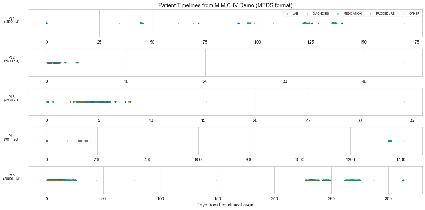
Each patient’s record is a sequence of events at irregular times. Compare this to tabular data (fixed columns) or regular time series (fixed intervals). EHR data has variable numbers of events, irregular timing, and mixed types.
Important: MEDS adds a BIRTH event at the patient’s date of birth. For timeline visualization we exclude this to focus on the clinical observation window.
## FIGURE — Patient Timelines from Real MIMIC-IV Data

color_map = {"LAB": PAL[0], "DIAGNOSIS": PAL[1], "MEDICATION": PAL[2],
             "PROCEDURE": PAL[3], "VITAL": PAL[4]}

# Pick 5 patients at different event-count quantiles
sorted_pts = events_per_patient.sort_values()
selected = [sorted_pts.index[int(q * len(sorted_pts))] for q in [0.1, 0.3, 0.5, 0.7, 0.9]]

fig, axes = plt.subplots(5, 1, figsize=(14, 7), sharex=False)
legend_shown = set()

for idx, (ax, pid) in enumerate(zip(axes, selected)):
    pt = clinical[clinical["subject_id"] == pid].copy()
    t0 = pt["time"].min()
    pt["days"] = (pt["time"] - t0).dt.total_seconds() / 86400

    for cat, color in color_map.items():
        subset = pt[pt["category"] == cat]
        if len(subset) == 0: continue
        label = cat if cat not in legend_shown else None
        ax.scatter(subset["days"], [0.5]*len(subset), c=[color], s=8, alpha=0.4,
                   label=label, zorder=3)
        legend_shown.add(cat)

    # Also show "other" categories in gray
    other = pt[~pt["category"].isin(color_map)]
    if len(other) > 0:
        label = "OTHER" if "OTHER" not in legend_shown else None
        ax.scatter(other["days"], [0.5]*len(other), c=["gray"], s=5, alpha=0.2,
                   label=label, zorder=2)
        legend_shown.add("OTHER")

    ax.set_yticks([])
    ax.set_ylabel(f"Pt {idx+1}\n({len(pt)} evt)", fontsize=8, rotation=0, labelpad=40)

axes[0].set_title("Patient Timelines from MIMIC-IV Demo (MEDS format)")
axes[-1].set_xlabel("Days from first clinical event")
axes[0].legend(loc="upper right", fontsize=7, ncol=6, framealpha=0.8)
plt.tight_layout()
plt.show()
3. Zipf’s Law in Medical Code Frequencies#
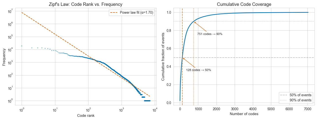
The number of “features” depends on code granularity. The underlying reason is Zipf’s law: a few codes are extremely common and most are very rare. This has direct implications for feature engineering and model design.
## FIGURE — Zipf's Law: Code Frequency Distribution

code_freq = clinical["code"].value_counts()
ranks = np.arange(1, len(code_freq) + 1)

fig, axes = plt.subplots(1, 2, figsize=(13, 5))

# Left: Rank-frequency (log-log)
ax = axes[0]
ax.loglog(ranks, code_freq.values, 'o', markersize=1.5, color=PAL[0], alpha=0.5)
# Power-law fit on top half
n_fit = len(ranks) // 2
slope, intercept = np.polyfit(np.log10(ranks[:n_fit]), np.log10(code_freq.values[:n_fit]), 1)
ax.loglog(ranks, 10**(intercept + slope * np.log10(ranks)), '--', color=PAL[3],
          label=f"Power law fit (α={-slope:.2f})")
ax.set_xlabel("Code rank"); ax.set_ylabel("Frequency")
ax.set_title("Zipf's Law: Code Rank vs. Frequency"); ax.legend()

# Right: Cumulative coverage
ax = axes[1]
cum = np.cumsum(code_freq.values) / code_freq.values.sum()
ax.plot(ranks, cum, color=PAL[0], linewidth=2)
ax.axhline(0.5, color="gray", ls="--", alpha=0.5, label="50% of events")
ax.axhline(0.9, color="gray", ls=":", alpha=0.5, label="90% of events")
n50 = np.searchsorted(cum, 0.5) + 1
n90 = np.searchsorted(cum, 0.9) + 1
ax.axvline(n50, color=PAL[3], ls="--", alpha=0.7)
ax.axvline(n90, color=PAL[3], ls=":", alpha=0.7)
ax.set_xlabel("Number of codes"); ax.set_ylabel("Cumulative fraction of events")
ax.set_title("Cumulative Code Coverage"); ax.legend()
ax.annotate(f"{n50} codes → 50%", xy=(n50, 0.5), fontsize=9,
            xytext=(n50+200, 0.35), arrowprops=dict(arrowstyle="->", color=PAL[3]))
ax.annotate(f"{n90} codes → 90%", xy=(n90, 0.9), fontsize=9,
            xytext=(n90+200, 0.75), arrowprops=dict(arrowstyle="->", color=PAL[3]))

plt.tight_layout(); plt.show()

print(f"Total unique codes: {len(code_freq)}")
print(f"Top {n50} codes ({n50/len(code_freq):.1%} of vocab) → 50% of events")
print(f"Top {n90} codes ({n90/len(code_freq):.1%} of vocab) → 90% of events")
print(f"This is Zipf's law: the long tail of rare codes is the 'curse of dimensionality'.")
Total unique codes: 7034
Top 128 codes (1.8% of vocab) → 50% of events
Top 751 codes (10.7% of vocab) → 90% of events
This is Zipf's law: the long tail of rare codes is the 'curse of dimensionality'.
4. Code Ontology and Feature Dimensionality#
The MEDS code format TYPE//ONTOLOGY//DETAIL naturally gives us multiple granularity levels. Using just the category (LAB, DIAGNOSIS, etc.) gives very few features; using full codes gives thousands. This is the “feature dimensionality is a design choice” point from the lecture.
## FIGURE — Feature Dimensionality at Different Granularity Levels

gran = {"Category\n(LAB, DX, ...)": clinical["category"],
        "Category//Ontology": clinical["code"].apply(lambda c: "//".join(str(c).split("//")[:2])),
        "Full code": clinical["code"]}

per_patient = {}
vocab_size = {}
for label, series in gran.items():
    per_patient[label] = series.groupby(clinical["subject_id"]).nunique().values
    vocab_size[label] = series.nunique()

fig, axes = plt.subplots(1, 2, figsize=(13, 5))

ax = axes[0]
bp = ax.boxplot([per_patient[l] for l in gran], tick_labels=list(gran.keys()),
                patch_artist=True, widths=0.5)
for patch, c in zip(bp["boxes"], [PAL[0], PAL[1], PAL[2]]):
    patch.set_facecolor(c); patch.set_alpha(0.6)
ax.set_ylabel("Unique codes per patient"); ax.set_yscale("log")
ax.set_title("Feature Dimensionality by Granularity")

ax = axes[1]
labels = list(gran.keys())
vals = [vocab_size[l] for l in gran]
bars = ax.bar(labels, vals, color=[PAL[0], PAL[1], PAL[2]], alpha=0.7)
for b, v in zip(bars, vals):
    ax.text(b.get_x() + b.get_width()/2., b.get_height() * 1.15, str(v), ha="center", fontsize=10)
ax.set_ylabel("Total unique codes"); ax.set_yscale("log")
ax.set_title("Vocabulary Size by Granularity")

plt.tight_layout(); plt.show()
print(f"Same 100 patients: {vals[0]} categories → {vals[1]} ontology-level → {vals[2]} full codes")
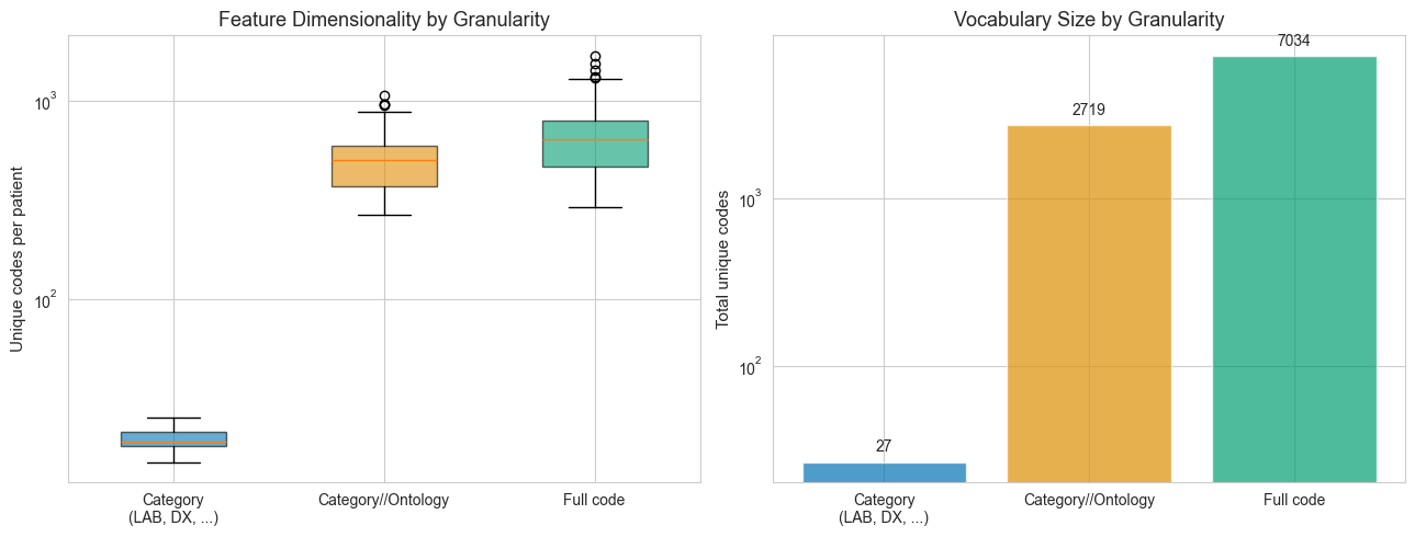
Same 100 patients: 27 categories → 2719 ontology-level → 7034 full codes
A Note on Code Hierarchies#
The MEDS codes.parquet metadata includes parent_codes for some codes, which enables
hierarchical aggregation. For example, ICD-9 code 4019 (Essential hypertension, unspecified)
has parent codes that map up through the ICD chapter hierarchy.
However, there are practical limitations for this demo:
Mixed ontologies: MIMIC-IV spans the ICD-9 → ICD-10 transition (Oct 2015), so some patients have ICD-9 codes (e.g.,
4019) and others have ICD-10 (e.g.,I10) for the same condition.Non-ICD codes: Lab codes (itemids like
220045) and procedure codes don’t share the ICD hierarchy.MEDS simplicity: MEDS intentionally stores flat
(subject_id, time, code, value)tuples. Hierarchical aggregation is a downstream choice, not baked into the format.
For a full ontology-based analysis, you would typically use tools like OMOP’s concept hierarchy
or the MEDS parent_codes metadata to roll up codes — but this adds complexity that may or may
not be warranted depending on your task. The granularity levels we showed above
(category → ontology → full code) are a simpler proxy that captures the key dimensionality trade-off.
## ICD Hierarchy via parent_codes (where available)

# Show how parent_codes can be used for hierarchical aggregation
if codes_files:
    # Find diagnosis codes with parent info
    dx_codes = codes_meta[codes_meta["code"].str.startswith("DIAGNOSIS")]
    dx_with_parents = dx_codes[dx_codes["parent_codes"].apply(
        lambda x: x is not None and len(x) > 0 if isinstance(x, (list, np.ndarray)) else False
    )]

    print(f"Diagnosis codes with parent hierarchy: {len(dx_with_parents)}/{len(dx_codes)}")
    print("\nExamples of ICD hierarchy in MEDS parent_codes:")
    for _, row in dx_with_parents.head(6).iterrows():
        name = resolve_code(row["code"])
        parents = row["parent_codes"]
        parent_names = [resolve_code(p) for p in parents] if isinstance(parents, (list, np.ndarray)) else []
        print(f"  {row['code']}")
        print(f"    Name: {name}")
        print(f"    Parents: {parents}")
        print()

    # Count how many hierarchy levels we get
    depths = dx_with_parents["parent_codes"].apply(
        lambda x: len(x) if isinstance(x, (list, np.ndarray)) else 0
    )
    print(f"Hierarchy depth: median={depths.median():.0f}, max={depths.max()}")
    print(f"\nNote: This hierarchy could create intermediate granularity levels")
    print(f"between 'category' and 'full code', but requires handling the")
    print(f"ICD-9/ICD-10 split and non-ICD code types.")
else:
    print("No codes.parquet found.")
Diagnosis codes with parent hierarchy: 1474/1474

Examples of ICD hierarchy in MEDS parent_codes:
  DIAGNOSIS//ICD//9//70723
    Name: 70723: Pressure ulcer, stage III
    Parents: ['ICD9CM/707.23']

  DIAGNOSIS//ICD//10//I951
    Name: I951: Orthostatic hypotension
    Parents: ['ICD10CM/I95.1']

  DIAGNOSIS//ICD//9//5778
    Name: 5778: Other specified diseases of pancreas
    Parents: ['ICD9CM/577.8']

  DIAGNOSIS//ICD//9//34831
    Name: 34831: Metabolic encephalopathy
    Parents: ['ICD9CM/348.31']

  DIAGNOSIS//ICD//10//F514
    Name: F514: Sleep terrors [night terrors]
    Parents: ['ICD10CM/F51.4']

  DIAGNOSIS//ICD//10//K521
    Name: K521: Toxic gastroenteritis and colitis
    Parents: ['ICD10CM/K52.1']

Hierarchy depth: median=1, max=1

Note: This hierarchy could create intermediate granularity levels
between 'category' and 'full code', but requires handling the
ICD-9/ICD-10 split and non-ICD code types.
5. Informative Observation#
Sicker patients generate more events. In MIMIC-IV all patients are ICU patients (already heavily selected), but there’s still substantial variation. We filter out the BIRTH event to compute the actual clinical observation window.
A Note on Mortality in MIMIC-IV Demo#
The MIMIC-III demo selected 100 patients who all died. The MIMIC-IV demo (v2.2) selected 100 patients for overlap with MIMIC-CXR — not based on mortality. So the survived/died split below is genuine for in-hospital mortality.
However, beware a subtle completeness issue: MIMIC-IV records out-of-hospital deaths in the
patients.dod column, but the MEDS ETL may not capture all of these as event codes. Some
patients labeled “survived” below may have died after discharge but lack a corresponding
death event in the MEDS stream. This is itself an example of the data completeness
challenges we discuss in the lecture.
## FIGURE — Informative Observation

pstats = clinical.groupby("subject_id").agg(
    n_events=("code", "size"),
    n_codes=("code", "nunique"),
    t_min=("time", "min"),
    t_max=("time", "max"),
).reset_index()
pstats["span_days"] = (pstats["t_max"] - pstats["t_min"]).dt.total_seconds() / 86400

# Check for death events
death_pids = set(clinical[clinical["code"].str.contains("DEATH|DISCHARGE_DEAD|death",
                                                         case=False, na=False)]["subject_id"])
pstats["died"] = pstats["subject_id"].isin(death_pids).astype(int)

fig, axes = plt.subplots(1, 3, figsize=(15, 4.5))

# Left: event count histogram (log scale)
ax = axes[0]
ax.hist(pstats["n_events"], bins=30, color=PAL[0], alpha=0.7, edgecolor="white")
ax.set_xlabel("Events per patient"); ax.set_ylabel("Count")
ax.set_title("Event Count Distribution"); ax.set_xscale("log")
ax.axvline(pstats["n_events"].median(), color=PAL[3], ls="--",
           label=f"Median: {pstats['n_events'].median():.0f}")
ax.legend()

# Middle: span vs events
ax = axes[1]
ax.scatter(pstats["span_days"], pstats["n_events"], alpha=0.5, s=30, c=PAL[0])
ax.set_xlabel("Clinical observation span (days)")
ax.set_ylabel("Number of events"); ax.set_yscale("log")
ax.set_title("Longer Stay → More Events")
r = pstats["span_days"].corr(pstats["n_events"])
ax.annotate(f"r = {r:.2f}", xy=(0.05, 0.95), xycoords="axes fraction", fontsize=11, fontweight="bold")

# Right: events by mortality
ax = axes[2]
if pstats["died"].sum() > 5:
    for val, label, col in [(0, "Survived", PAL[0]), (1, "Died", PAL[3])]:
        subset = pstats[pstats["died"] == val]["n_events"]
        ax.hist(subset, bins=20, alpha=0.5, label=f"{label} (n={len(subset)})",
                color=col, edgecolor="white")
    ax.set_xlabel("Events per patient"); ax.set_ylabel("Count")
    ax.set_title("Events by Mortality"); ax.set_xscale("log"); ax.legend()
else:
    ax.text(0.5, 0.5, f"Only {pstats['died'].sum()} deaths\nidentified by code",
            transform=ax.transAxes, ha="center", fontsize=11)
    ax.set_title("Events by Mortality")

plt.tight_layout(); plt.show()

print(f"Observation spans: median={pstats['span_days'].median():.1f} days, "
      f"mean={pstats['span_days'].mean():.1f} days")
print(f"(Compare to the ~65-year spans if we include the BIRTH event!)")
print(f"Span-event correlation: r={r:.2f}")
if pstats['died'].sum() > 0:
    print(f"Deaths identified: {pstats['died'].sum()}/{len(pstats)} patients")
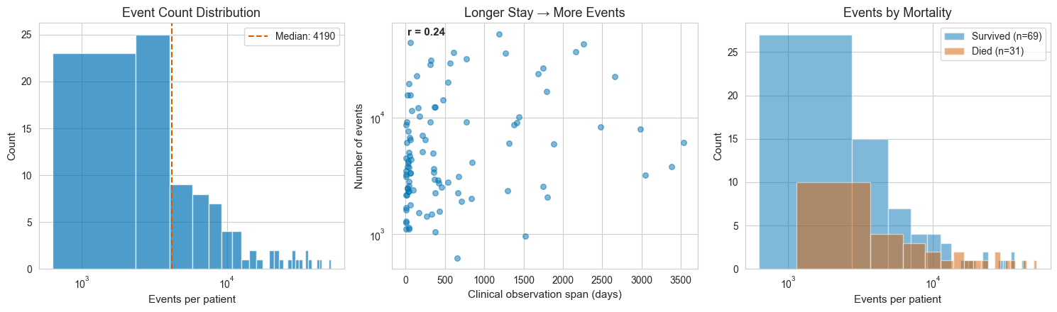
Observation spans: median=313.0 days, mean=614.2 days
(Compare to the ~65-year spans if we include the BIRTH event!)
Span-event correlation: r=0.24
Deaths identified: 31/100 patients
6. Berkson’s Paradox in Real Data#
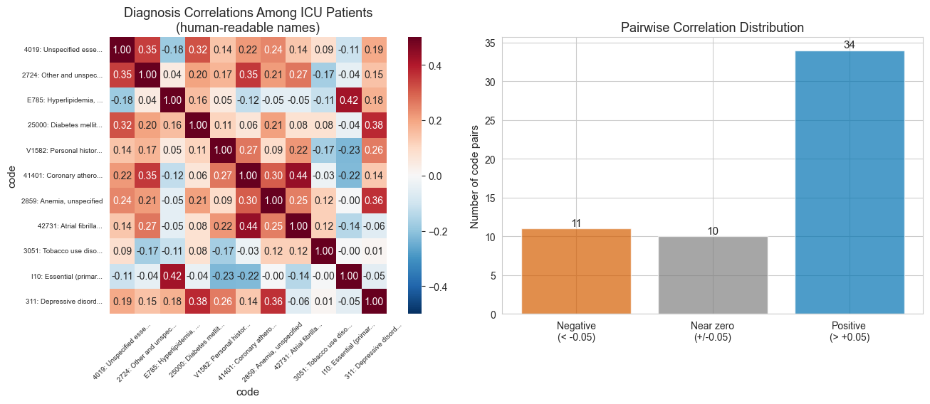
All 100 patients are ICU patients — conditioned on being severely ill. Any correlations we see between diagnoses may not reflect population-level associations.
We look for diagnosis pairs that show negative correlations — these are candidates for Berkson’s bias, where one condition “explains away” why the patient is in the ICU.
## FIGURE — Berkson's Paradox: Diagnosis Correlations Among ICU Patients

dx = clinical[clinical["category"] == "DIAGNOSIS"].copy()
print(f"Diagnosis events: {len(dx):,} | Unique codes: {dx['code'].nunique()}")

# Build patient x diagnosis binary matrix
dx_binary = dx.groupby(["subject_id", "code"]).size().reset_index(name="n")
dx_pivot = dx_binary.pivot_table(index="subject_id", columns="code", values="n", fill_value=0)
dx_present = (dx_pivot > 0).astype(int)

# Find codes with 15-85% prevalence (interesting variance)
prev = dx_present.mean()
interesting = prev[(prev > 0.15) & (prev < 0.85)].sort_values(ascending=False)
print(f"Codes with 15-85% prevalence: {len(interesting)}")

if len(interesting) >= 4:
    top = interesting.head(min(12, len(interesting)))
    subset = dx_present[top.index]
    corr = subset.corr()

    # Resolve to human-readable names
    short_names = []
    for c in corr.columns:
        name = resolve_code(c)
        if len(name) > 25:
            name = name[:22] + "..."
        short_names.append(name)

    # Print the code-to-name mapping for reference
    print("\nCode legend:")
    for c, name in zip(corr.columns, short_names):
        full_name = resolve_code(c)
        prev_val = prev[c]
        print(f"  {name:25s} (prev: {prev_val:.0%}) <- {c}")

    fig, axes = plt.subplots(1, 2, figsize=(14, 5.5))

    ax = axes[0]
    sns.heatmap(corr, annot=True, fmt=".2f", cmap="RdBu_r", center=0,
                xticklabels=short_names, yticklabels=short_names,
                ax=ax, vmin=-0.5, vmax=0.5, square=True)
    ax.set_title("Diagnosis Correlations Among ICU Patients\n(human-readable names)")
    ax.tick_params(axis='x', rotation=45, labelsize=7)
    ax.tick_params(axis='y', rotation=0, labelsize=7)

    ax = axes[1]
    upper = corr.where(np.triu(np.ones_like(corr, dtype=bool), k=1))
    n_neg = (upper < -0.05).sum().sum()
    n_zero = (upper.abs() <= 0.05).sum().sum()
    n_pos = (upper > 0.05).sum().sum()
    bars = ax.bar(["Negative\n(< -0.05)", "Near zero\n(+/-0.05)", "Positive\n(> +0.05)"],
                  [n_neg, n_zero, n_pos], color=[PAL[3], "gray", PAL[0]], alpha=0.7)
    for b, v in zip(bars, [n_neg, n_zero, n_pos]):
        ax.text(b.get_x()+b.get_width()/2., b.get_height()+0.3, str(v), ha="center", fontsize=11)
    ax.set_ylabel("Number of code pairs")
    ax.set_title("Pairwise Correlation Distribution")

    plt.tight_layout()
    plt.show()

    # Highlight the most negative pairs (strongest Berkson's candidates)
    print(f"\n{'='*60}")
    print(f"BERKSON'S PARADOX CANDIDATES (most negative correlations):")
    print(f"{'='*60}")
    pairs = []
    for ci in range(len(corr.columns)):
        for cj in range(ci+1, len(corr.columns)):
            r = corr.iloc[ci, cj]
            pairs.append((r, corr.columns[ci], corr.columns[cj]))
    pairs.sort()

    for r, c1, c2 in pairs[:5]:
        n1 = resolve_code(c1)
        n2 = resolve_code(c2)
        print(f"  r = {r:+.2f}: {n1}  x  {n2}")
        print(f"         The negative correlation may be an artifact of")
        print(f"         conditioning on ICU admission (Berkson's Paradox).\n")
Diagnosis events: 4,506 | Unique codes: 1474
Codes with 15-85% prevalence: 11

Code legend:
  4019: Unspecified esse... (prev: 41%) <- DIAGNOSIS//ICD//9//4019
  2724: Other and unspec... (prev: 34%) <- DIAGNOSIS//ICD//9//2724
  E785: Hyperlipidemia, ... (prev: 21%) <- DIAGNOSIS//ICD//10//E785
  25000: Diabetes mellit... (prev: 21%) <- DIAGNOSIS//ICD//9//25000
  V1582: Personal histor... (prev: 20%) <- DIAGNOSIS//ICD//9//V1582
  41401: Coronary athero... (prev: 19%) <- DIAGNOSIS//ICD//9//41401
  2859: Anemia, unspecified (prev: 18%) <- DIAGNOSIS//ICD//9//2859
  42731: Atrial fibrilla... (prev: 18%) <- DIAGNOSIS//ICD//9//42731
  3051: Tobacco use diso... (prev: 18%) <- DIAGNOSIS//ICD//9//3051
  I10: Essential (primar... (prev: 17%) <- DIAGNOSIS//ICD//10//I10
  311: Depressive disord... (prev: 16%) <- DIAGNOSIS//ICD//9//311
============================================================
BERKSON'S PARADOX CANDIDATES (most negative correlations):
============================================================
  r = -0.23: V1582: Personal history of tobacco use  x  I10: Essential (primary) hypertension
         The negative correlation may be an artifact of
         conditioning on ICU admission (Berkson's Paradox).

  r = -0.22: 41401: Coronary atherosclerosis of native coronary artery  x  I10: Essential (primary) hypertension
         The negative correlation may be an artifact of
         conditioning on ICU admission (Berkson's Paradox).

  r = -0.18: 4019: Unspecified essential hypertension  x  E785: Hyperlipidemia, unspecified
         The negative correlation may be an artifact of
         conditioning on ICU admission (Berkson's Paradox).

  r = -0.17: 2724: Other and unspecified hyperlipidemia  x  3051: Tobacco use disorder
         The negative correlation may be an artifact of
         conditioning on ICU admission (Berkson's Paradox).

  r = -0.17: V1582: Personal history of tobacco use  x  3051: Tobacco use disorder
         The negative correlation may be an artifact of
         conditioning on ICU admission (Berkson's Paradox).
7. EHR vs. Claims: Simulating Information Loss#
We simulate a claims-like view by keeping only diagnosis codes and aggregating to daily level. This mimics what a payer sees vs. what the hospital EHR contains.
## EHR → Claims Transformation

dx_only = clinical[clinical["category"] == "DIAGNOSIS"].copy()
dx_only["date"] = dx_only["time"].dt.date

claims_view = dx_only.groupby(["subject_id", "date"]).agg(
    codes=("code", lambda x: list(x.unique())),
    n_codes=("code", "nunique")
).reset_index()

print(f"EHR view:    {len(clinical):,} individual events across all types")
print(f"Claims view: {len(claims_view):,} daily claim records (diagnosis only)")
print(f"Compression: {len(clinical) / max(len(claims_view), 1):.0f}x")
print(f"\nWhat's lost:")
print(f"  Lab values:    {clinical['numeric_value'].notna().sum():,} numeric measurements → gone")
print(f"  Vital signs:   {(clinical['category']=='VITAL').sum():,} events → gone")
print(f"  Medications:   {(clinical['category']=='MEDICATION').sum():,} events → gone")
print(f"  Temporal grain: minute-level → day-level")
EHR view:    916,066 individual events across all types
Claims view: 275 daily claim records (diagnosis only)
Compression: 3331x

What's lost:
  Lab values:    405,236 numeric measurements → gone
  Vital signs:   0 events → gone
  Medications:   63,696 events → gone
  Temporal grain: minute-level → day-level
## FIGURE — Feature Comparison: EHR vs Claims

def make_ehr_features(pid_events):
    f = {}
    f["n_events"] = len(pid_events)
    f["n_codes"] = pid_events["code"].nunique()
    for cat in ["LAB", "DIAGNOSIS", "MEDICATION", "PROCEDURE", "VITAL"]:
        f[f"n_{cat}"] = (pid_events["category"] == cat).sum()
    nums = pid_events["numeric_value"].dropna()
    f["n_numeric"] = len(nums)
    f["numeric_mean"] = nums.mean() if len(nums) > 0 else 0
    f["numeric_std"] = nums.std() if len(nums) > 1 else 0
    span = (pid_events["time"].max() - pid_events["time"].min()).total_seconds() / 86400
    f["span_days"] = span
    return f

def make_claims_features(pid_claims):
    f = {}
    all_codes = []
    for cl in pid_claims["codes"]:
        all_codes.extend(cl)
    f["n_claims"] = len(pid_claims)
    f["n_codes"] = len(set(all_codes))
    return f

pids = sorted(clinical["subject_id"].unique())
X_ehr = pd.DataFrame([make_ehr_features(clinical[clinical["subject_id"]==p]) for p in pids]).fillna(0)
X_claims = pd.DataFrame([make_claims_features(claims_view[claims_view["subject_id"]==p]) for p in pids]).fillna(0)

fig, ax = plt.subplots(figsize=(10, 4))
labels = list(X_ehr.columns)
ehr_vals = X_ehr.mean()
ax.barh(range(len(labels)), ehr_vals, color=PAL[0], alpha=0.7, label="EHR features")
ax.set_yticks(range(len(labels))); ax.set_yticklabels(labels, fontsize=8)
ax.set_xlabel("Mean value per patient"); ax.set_xscale("log")
ax.set_title(f"EHR: {X_ehr.shape[1]} features | Claims: {X_claims.shape[1]} features")
ax.legend(); plt.tight_layout(); plt.show()

print(f"EHR features:    {X_ehr.shape[1]} dimensions")
print(f"Claims features: {X_claims.shape[1]} dimensions")
print(f"Information ratio: {X_ehr.shape[1]/X_claims.shape[1]:.1f}x more features in EHR")
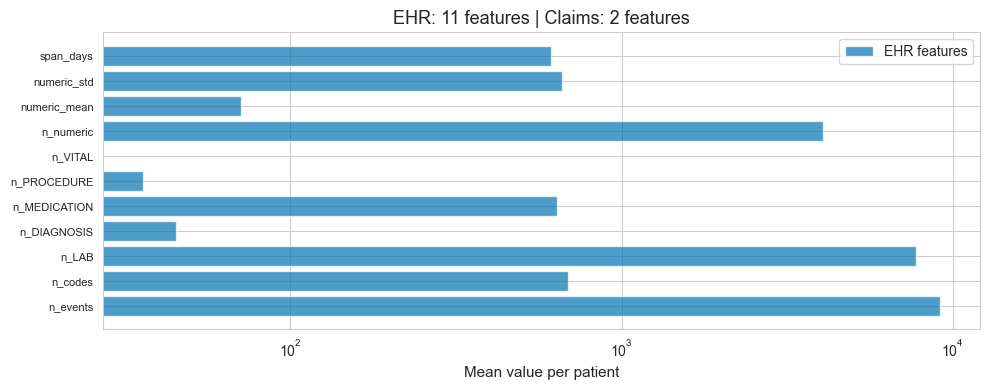
EHR features:    11 dimensions
Claims features: 2 dimensions
Information ratio: 5.5x more features in EHR
8. Censoring and Observation Windows#
All 100 patients are ICU patients. Their records start at hospital admission and end at discharge or death. We have no data about their health before or after.
Note: We exclude the BIRTH event (which MEDS places at the patient’s date of birth) — otherwise observation spans appear to be ~65 years rather than the actual ICU stay duration.
## FIGURE — Observation Windows and Inter-Event Times

fig, axes = plt.subplots(1, 2, figsize=(14, 5))

# Left: Observation windows sorted by span
ax = axes[0]
ss = pstats.sort_values("span_days").reset_index(drop=True)
colors = [PAL[3] if d else PAL[0] for d in ss["died"]]
for i, row in ss.iterrows():
    ax.barh(i, row["span_days"], height=0.8, color=colors[i], alpha=0.5)
ax.set_xlabel("Clinical observation span (days)")
ax.set_ylabel("Patient (sorted by span)")
ax.set_title("Observation Windows (excluding birth event)")
ax.axvline(ss["span_days"].median(), color="gray", ls="--",
           label=f"Median: {ss['span_days'].median():.0f} days")
survived_patch = mpatches.Patch(color=PAL[0], alpha=0.5, label="Survived")
died_patch = mpatches.Patch(color=PAL[3], alpha=0.5, label="Died")
ax.legend(handles=[survived_patch, died_patch, ax.get_lines()[0]], fontsize=8)

# Right: Inter-event time distribution (LOG SCALE)
ax = axes[1]
iet_all = []
for pid, grp in clinical.groupby("subject_id"):
    t = grp["time"].sort_values()
    if len(t) > 1:
        gaps = t.diff().dropna().dt.total_seconds() / 3600  # hours
        iet_all.extend(gaps.values)

iet = np.array(iet_all)
iet_pos = iet[iet > 0]  # exclude simultaneous events for log scale

ax.hist(np.log10(iet_pos + 1e-3), bins=80, color=PAL[0], alpha=0.7, edgecolor="white", density=True)
ax.set_xlabel("Inter-event time (log₁₀ hours)")
ax.set_ylabel("Density")
ax.set_title("Inter-Event Time Distribution (log scale)")

# Add reference lines
for val, label in [(0, "1 hour"), (np.log10(24), "1 day"), (np.log10(168), "1 week")]:
    ax.axvline(val, color=PAL[3], ls="--", alpha=0.5)
    ax.text(val+0.05, ax.get_ylim()[1]*0.9, label, fontsize=7, color=PAL[3])

pct_zero = (iet == 0).mean()
ax.annotate(f"{pct_zero:.0%} of gaps\nare 0 hours\n(simultaneous events)",
            xy=(0.02, 0.6), xycoords="axes fraction", fontsize=9,
            bbox=dict(boxstyle="round", fc="lightyellow", alpha=0.8))

plt.tight_layout(); plt.show()

print(f"Inter-event times: {pct_zero:.1%} are exactly 0 (simultaneous)")
print(f"  Median (non-zero): {np.median(iet_pos):.2f} hours")
print(f"  Mean (non-zero): {np.mean(iet_pos):.1f} hours")
print(f"\nICU data is DENSE — most events happen within the same hour.")
print(f"This is very different from outpatient data where gaps are weeks/months.")
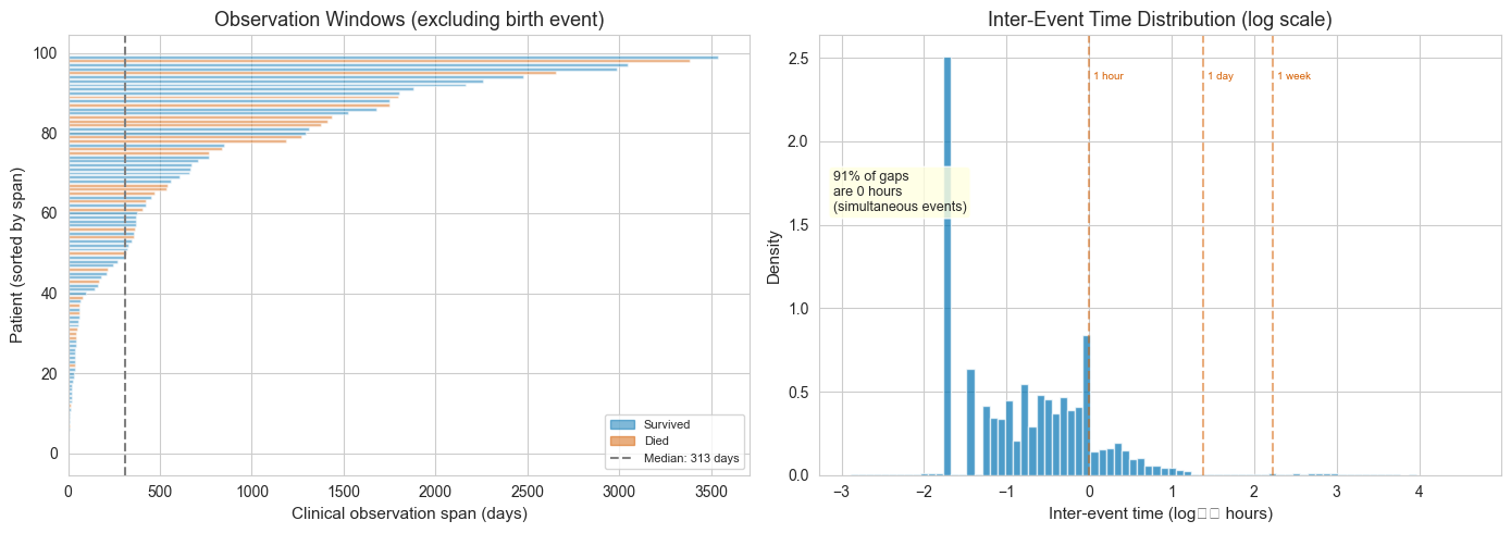
Inter-event times: 90.9% are exactly 0 (simultaneous)
  Median (non-zero): 0.17 hours
  Mean (non-zero): 17.7 hours

ICU data is DENSE — most events happen within the same hour.
This is very different from outpatient data where gaps are weeks/months.
Discussion Questions#
Berkson’s Paradox: Look at the most negative diagnosis pairs above. For each one, consider: is there a plausible biological reason for negative correlation, or is this more likely Berkson’s bias? How would you test this?
Mortality completeness: We found ~31 in-hospital deaths, but the MIMIC-III demo (same size) had 100% mortality by design. The MIMIC-IV demo wasn’t selected on mortality, but some “survivors” may have died after discharge with no death event in MEDS. What does this tell you about using MEDS death codes as ground truth for a mortality prediction task?
Zipf’s law: The top ~100 codes cover 50% of events, but rare codes may carry the most clinical information. How would you handle this for feature engineering?
ICD hierarchy: We showed that MEDS
parent_codescan enable hierarchical aggregation, but the ICD-9/ICD-10 split complicates this. When would it be worth the effort to build a proper ontology-based feature hierarchy vs. just using the MEDS category/ontology levels?Censoring: MIMIC only covers hospital stays. If predicting 30-day readmission, what problems arise from missing outpatient data between admissions?
MEDS format: What are the advantages and limitations of
(subject_id, time, code, value)tuples? What clinical info is hard to capture in this flat format?
Data Reference#
Statistic |
Value |
|---|---|
Patients |
100 (ICU) |
Total events |
~916K |
Clinical events (excl. birth) |
~916K |
Unique codes |
~7,000 |
Median events/patient |
~4,200 |
Median observation span |
varies (days) |
Event types |
LAB, DIAGNOSIS, MEDICATION, PROCEDURE, VITAL, … |
Citation: Johnson et al., MIMIC-IV (PhysioNet). McDermott et al., Medical Event Data Standard (MEDS).