🧠 Lab 5: Neural Networks – Multi-Layer Perceptron

🧠 Lab 5: Neural Networks – Multi-Layer Perceptron#

BINF 4002 – Machine Learning for Health

Learning Objectives#

Understand how a multi-layer perceptron works mathematically, from neurons to layers to backpropagation
Implement the forward pass yourself and verify it against sklearn
Understand activation functions and why choice matters
Observe training dynamics: loss curves, learning rate effects, and overfitting in real time
Understand and demonstrate dropout as a regularization strategy
Recognize and fix the calibration problem unique to neural networks
Compare MLPs to simpler models – and know when neural networks don’t help

⚠️ This is a basic intro to neural networks. We’ll see more complex networks and more advanced training techniques and information later in the course. Not all of these lessons will scale up to very large scale models!

What Is a Neural Network?#

A multi-layer perceptron (MLP) is a sequence of layers, where each layer applies a learned linear transformation followed by a non-linear activation function. The key insight is that composing enough of these simple operations can approximate arbitrarily complex functions – the universal approximation theorem.

From neurons to layers#

A single neuron takes a vector input $\mathbf{x} \in \mathbb{R}^d$, computes a weighted sum, adds a bias, and applies an activation:

\[a = \sigma(\mathbf{w}^\top \mathbf{x} + b)\]

A layer is simply $h$ neurons in parallel, sharing the same input but with different weights. We collect all $h$ weight vectors into a matrix $W \in \mathbb{R}^{d \times h}$ and all biases into $\mathbf{b} \in \mathbb{R}^h$:

\[\mathbf{a} = \sigma(W^\top \mathbf{x} + \mathbf{b})\]

(applied element-wise to the activation). For a batch of $n$ samples as rows in $X \in \mathbb{R}^{n \times d}$:

\[A = \sigma(X W + \mathbf{b}) \in \mathbb{R}^{n \times h}\]

Recall the ‘linear combination of columns’ perspective on matrix multiplication to help see how $\mathbf w$ in the formula for $a$ and $W$ in the formula for $\mathbf{a}$ relate.

The 2-layer MLP we’ll implement#

\[\underbrace{X}_{n \times d} \xrightarrow{\text{Linear}} Z_1 = XW_1 + b_1 \xrightarrow{\text{ReLU}} A_1 = \text{ReLU}(Z_1) \xrightarrow{\text{Linear}} Z_2 = A_1 W_2 + b_2 \xrightarrow{\text{Sigmoid}} \hat{p} = \sigma(Z_2)\]

The output $\hat{p}_i \in (0, 1)$ is the estimated probability $P(Y=1 \mid \mathbf{x}_i)$.

Training: loss and backpropagation#

The network is trained by minimizing binary cross-entropy loss over the training set:

\[\mathcal{L} = -\frac{1}{n}\sum_{i=1}^n \left[ y_i \log \hat{p}_i + (1-y_i)\log(1-\hat{p}_i) \right]\]

Question: Why is this loss reasonable? How does this compare to the loss that you might use to train a logistic regression model, were you to train it via gradient descent?

Minimization is done by gradient descent: compute $\nabla_W \mathcal{L}$ via backpropagation (the chain rule applied layer by layer, from output to input), then update each weight:

\[W \leftarrow W - \eta \nabla_W \mathcal{L}\]

where $\eta$ is the learning rate. This repeats for many epochs (passes through the training data). In this lab, we use sklearn’s implementation, which does this automatically – but we will implement the forward pass ourselves to confirm we understand the math.

When do neural networks add value?#

Neural networks excel when:

$n$ is large (typically $n > 10{,}000$): the model has enough parameters to overfit easily, and enough data to generalize despite it (recall the lecture on interpolation vs. memorization).
Inputs have structure: images (CNNs), sequences (RNNs/Transformers), graphs (GNNs), and more (We’ll see more about different types of data later in the course).
Non-linear interactions are complex and numerous: raw pixels, tokens, waveforms

For our small tabular dataset ($n=120$, $d=8$), neural networks may not outperform simpler models. This is an intentional lesson: more complex $\neq$ better.

Dataset: Restricted breast cancer features – 8 weakest features, 120 training samples

Set-up#

Upload data#

⚠️ First, you need to upload the pre-processed data from lab0. If you have issues with running the first lab, you can also download the data here.

Once you have downloaded the data locally and started the runtime for this ntoebook, upload the file to this notebook via the “Files” menu.

import os

pkl_path = 'processed_data.pkl'
if os.path.exists(pkl_path):
    print("✅ Data File Found!")
else:
    raise FileNotFoundError(
        "processed_data.pkl not found! "
        "Make sure you have run Lab 0 (lab0_preprocessing.ipynb) in full and "
        "downloaded the output (or used the link above), and uploaded it here."
    )

✅ Data File Found!

Imports and Helpers#

import os, pickle, warnings
import numpy as np
import pandas as pd
import matplotlib.pyplot as plt
import seaborn as sns
warnings.filterwarnings('ignore')

plt.rcParams['figure.dpi'] = 110
plt.rcParams['axes.spines.top'] = False
plt.rcParams['axes.spines.right'] = False

pkl_path = 'processed_data.pkl'
if not os.path.exists(pkl_path):
    raise FileNotFoundError(
        "processed_data.pkl not found. Run Lab 0 first, or download from the link above."
    )

with open(pkl_path, 'rb') as f:
    d = pickle.load(f)

X_train = d['X_train_hard'];  y_train = d['y_train_hard']
X_val   = d['X_val_hard'];    y_val   = d['y_val_hard']
X_test  = d['X_test_hard'];   y_test  = d['y_test_hard']
feature_names = d['feature_names_hard']
class_names   = ['Malignant', 'Benign']
n_features    = X_train.shape[1]

print(f"Train : {X_train.shape}  |  Val : {X_val.shape}  |  Test : {X_test.shape}")
print(f"n_features = {n_features}  (d=8 restricted features)")
print(f"Features: {feature_names}")
print(f"Training prevalence (fraction benign): {y_train.mean():.2%}")
print()
print("Note: 8 LEAST individually-informative features + 120 training samples.")
print("Expected AUC range: ~0.80-0.88  (realistic; not the trivial 0.99 of all features).")

Train : (100, 8)  |  Val : (114, 8)  |  Test : (114, 8)
n_features = 8  (d=8 restricted features)
Features: ['mean symmetry', 'compactness error', 'concavity error', 'smoothness error', 'texture error', 'fractal dimension error', 'symmetry error', 'mean fractal dimension']
Training prevalence (fraction benign): 60.00%

Note: 8 LEAST individually-informative features + 120 training samples.
Expected AUC range: ~0.80-0.88  (realistic; not the trivial 0.99 of all features).

from sklearn.neural_network import MLPClassifier
from sklearn.linear_model import LogisticRegression
from sklearn.metrics import confusion_matrix, roc_auc_score, roc_curve, auc
import warnings; warnings.filterwarnings('ignore')

def print_metrics(y_true, y_pred, y_prob=None, label='Model'):
    tn,fp,fn,tp = confusion_matrix(y_true, y_pred).ravel()
    n = len(y_true)
    sens = tp/(tp+fn); spec = tn/(tn+fp)
    ppv  = tp/(tp+fp); npv  = tn/(tn+fn)
    prev = (tp+fn)/n
    print(f"{'─'*55}")
    print(f"  {label}")
    print(f"{'─'*55}")
    print(f"  Sensitivity  P(ŷ=1|y=1)  = {tp}/{tp+fn} = {sens:.3f}")
    print(f"  Specificity  P(ŷ=0|y=0)  = {tn}/{tn+fp} = {spec:.3f}")
    print(f"  PPV          P(y=1|ŷ=1)  = {tp}/{tp+fp} = {ppv:.3f}")
    print(f"  NPV          P(y=0|ŷ=0)  = {tn}/{tn+fn} = {npv:.3f}")
    if y_prob is not None:
        print(f"  AUC-ROC                  = {roc_auc_score(y_true, y_prob):.3f}")
    print(f"  Prevalence               = {prev:.3f}")
    print()

def decision_curve(y_true, y_prob, thresholds=None, label='Model', ax=None, color='#3498db'):
    if thresholds is None:
        thresholds = np.linspace(0.01, 0.99, 150)
    prev = y_true.mean()
    nb_model, nb_all = [], []
    for t in thresholds:
        y_hat = (y_prob >= t).astype(int)
        tp = ((y_hat==1)&(y_true==1)).sum()
        fp = ((y_hat==1)&(y_true==0)).sum()
        n  = len(y_true)
        nb_model.append(tp/n - fp/n * t/(1-t))
        nb_all.append(prev - (1-prev)*t/(1-t))
    ax = ax or plt.gca()
    ax.plot(thresholds, nb_model, lw=2, label=label, color=color)
    ax.plot(thresholds, nb_all, 'k--', lw=1, alpha=0.5,
            label='Treat all' if label == 'Model' else '')
    ax.axhline(0, color='grey', lw=1, alpha=0.5)
    ax.set_xlabel('Probability threshold'); ax.set_ylabel('Net Benefit')
    ax.set_ylim(-0.05, prev + 0.05)
    return np.array(nb_model)

Part 1 – Activation Functions and the Forward Pass#

Activation functions#

The choice of activation function profoundly affects how a network trains and what it can represent. The two most important ones for this lab:

ReLU (Rectified Linear Unit): $$\text{ReLU}(z) = \max(0, z)$$ ReLU is the default choice for hidden layers in modern networks. It is computationally cheap, does not saturate for positive inputs (so gradients flow freely), and naturally produces sparse activations (negative pre-activations become exactly zero). The main risk is “dead neurons”: if a neuron’s pre-activation is always negative (e.g., after a large weight update), its gradient is permanently zero and it can never recover.

Sigmoid: $$\sigma(z) = \frac{1}{1 + e^{-z}}$$ Used *only* at the output layer for binary classification, to map the final linear value into a probability. Using sigmoid in hidden layers causes the **vanishing gradient problem**: when $|z|$ is large, $\sigma’(z) \approx 0$, so gradients approaching zero through many sigmoid layers prevent early layers from learning at all.

Below we visualize both before implementing the forward pass.

# Visualize activation functions and their gradients
z = np.linspace(-4, 4, 300)

relu_z    = np.maximum(0, z)
sigmoid_z = 1 / (1 + np.exp(-z))

# Gradients (derivatives)
drelu_z    = (z > 0).astype(float)
dsigmoid_z = sigmoid_z * (1 - sigmoid_z)

fig, axes = plt.subplots(2, 2, figsize=(14, 8))

axes[0,0].plot(z, relu_z, color='#e74c3c', lw=2.5)
axes[0,0].set_title('ReLU: max(0, z)', fontsize=12)
axes[0,0].set_ylabel('Activation'); axes[0,0].grid(True, alpha=0.3)
axes[0,0].axvline(0, color='grey', lw=0.8, linestyle='--')
axes[0,0].fill_between(z, relu_z, alpha=0.1, color='#e74c3c')
axes[0,0].annotate('Dead zone\n(gradient=0)', xy=(-2, 0.5),
                    fontsize=9, color='grey')

axes[0,1].plot(z, sigmoid_z, color='#3498db', lw=2.5)
axes[0,1].set_title('Sigmoid: 1/(1+exp(-z))', fontsize=12)
axes[0,1].set_ylabel('Activation'); axes[0,1].grid(True, alpha=0.3)
axes[0,1].axhline(0.5, color='grey', lw=0.8, linestyle='--', label='y=0.5')
axes[0,1].fill_between(z[z>2],  sigmoid_z[z>2],  1, alpha=0.15, color='orange', label='Saturation zones')
axes[0,1].fill_between(z[z<-2], sigmoid_z[z<-2], 0, alpha=0.15, color='orange')
axes[0,1].legend(fontsize=8)

axes[1,0].plot(z, drelu_z, color='#e74c3c', lw=2.5, drawstyle='steps-mid')
axes[1,0].set_title('ReLU gradient: 0 or 1 (never vanishes for z>0)', fontsize=11)
axes[1,0].set_ylabel("d(ReLU)/dz"); axes[1,0].set_ylim(-0.1, 1.5)
axes[1,0].grid(True, alpha=0.3)

axes[1,1].plot(z, dsigmoid_z, color='#3498db', lw=2.5)
axes[1,1].set_title('Sigmoid gradient: max 0.25 -- vanishes at extremes', fontsize=11)
axes[1,1].set_ylabel("d(sigmoid)/dz"); axes[1,1].grid(True, alpha=0.3)
axes[1,1].annotate('Max gradient = 0.25\nat z=0', xy=(0, 0.25),
                    xytext=(1.5, 0.22), arrowprops=dict(arrowstyle='->'), fontsize=9)
axes[1,1].fill_between(z[z>2],  dsigmoid_z[z>2],  alpha=0.3, color='orange', label='Near-zero gradient')
axes[1,1].fill_between(z[z<-2], dsigmoid_z[z<-2], alpha=0.3, color='orange')
axes[1,1].legend(fontsize=8)

for ax in axes.ravel():
    ax.set_xlabel('z (pre-activation)')
plt.suptitle('Activation Functions and Their Gradients', fontsize=13, y=1.01)
plt.tight_layout(); plt.show()

print("Key takeaways:")
print("  ReLU: gradient is exactly 1 for z>0, 0 for z<=0. No vanishing.")
print("  Sigmoid: gradient max is 0.25. At z=±4, gradient ≈ 0.018 -- nearly zero.")
print("  With 5 sigmoid layers, gradient can shrink by 0.25^5 ≈ 0.001 -- effectively gone.")

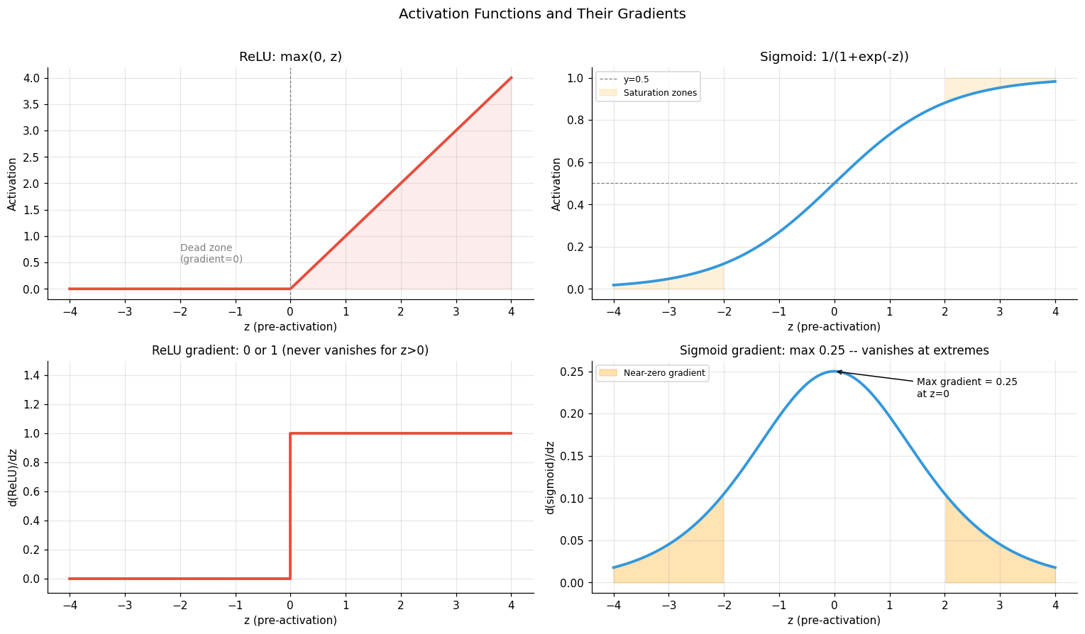
../_images/b07d6797f5bddb0ea9c4295856cd18d37cc15e7f7408b0402b8f0713412f8321.png

Key takeaways:
  ReLU: gradient is exactly 1 for z>0, 0 for z<=0. No vanishing.
  Sigmoid: gradient max is 0.25. At z=±4, gradient ≈ 0.018 -- nearly zero.
  With 5 sigmoid layers, gradient can shrink by 0.25^5 ≈ 0.001 -- effectively gone.

Questions:

What are some other activation functions you could imagine using?
What would go wrong if your activation function were linear?
Suppose I use a ReLU activation function, but all my neural network layer weights/biases are negative and all my feature values are positive. What problem might I encounter? What about if all my weights/biases are positive and all my feature values are positive?

✅ Solution — Activation Function Questions#

1. Other activation functions: Tanh: $\tanh(z) = (e^z - e^{-z})/(e^z + e^{-z})$, maps to $(-1, 1)$, zero-centered but still saturates. Leaky ReLU: $f(z) = z$ if $z > 0$, $\alpha z$ otherwise (small slope for negative inputs, avoids dead neurons). GELU (Gaussian Error Linear Unit): smooth approximation to ReLU used in transformers. Swish/SiLU: $f(z) = z \cdot \sigma(z)$, smooth and non-monotonic. Softplus: $f(z) = \log(1 + e^z)$, smooth approximation to ReLU.

2. Linear activation: If the activation is linear ($f(z) = z$), then composing multiple layers gives: $A_2 = (XW_1 + b_1)W_2 + b_2 = X(W_1 W_2) + (b_1 W_2 + b_2)$. This is just a single linear transformation with effective weights $W = W_1 W_2$ and bias $b = b_1 W_2 + b_2$. No matter how many layers you stack, the result is always a linear function of $X$. The network cannot learn any non-linear patterns — it collapses to logistic regression.

3. If all weights/biases are negative and all features are positive: $z_1 = XW_1 + b_1$ will be negative for every neuron (negative weights × positive inputs + negative bias). With ReLU, $a_1 = \max(0, z_1) = 0$ for every neuron — the entire hidden layer is dead. The network outputs a constant (just the bias of the output layer). If all weights/biases are positive and all features are positive: all pre-activations are positive, so ReLU passes everything through. The network functions normally, but all neurons compute similar (positive-weighted) combinations of the input, reducing representational diversity.

Implement the Forward Pass#

Now implement the forward pass using the math from the intro.

Architecture: Input ($d=8$) → Linear → ReLU → Linear → Sigmoid → $\hat{p}$

With hidden layer size $h=32$, the weight dimensions are:

$W_1 \in \mathbb{R}^{8 \times 32}$, $\mathbf{b}_1 \in \mathbb{R}^{32}$
$W_2 \in \mathbb{R}^{32 \times 1}$, $\mathbf{b}_2 \in \mathbb{R}^{1}$

Parameter count: $8 \times 32 + 32 + 32 \times 1 + 1 = 257 + 33 = \mathbf{322}$ parameters for 120 training samples. That is fewer than 1 sample per parameter – a very tight fit.

# ── SOLUTION ──────────────────────────────────────────────────────────────────
# Implement the forward pass of a 2-layer MLP.

def relu(z):
    # ReLU: max(0, z) -- apply element-wise.
    return np.maximum(0, z)

def sigmoid(z):
    # Sigmoid: 1 / (1 + exp(-z)) -- apply element-wise.
    return 1 / (1 + np.exp(-z))

def mlp_forward_pass(X, W1, b1, W2, b2):
    # 2-layer MLP forward pass.
    # X: (n_samples, n_features)  W1: (n_features, n_hidden)  b1: (n_hidden,)
    # W2: (n_hidden, 1)  b2: (1,)  Returns: (n_samples,) predicted P(Y=1|X)
    z1    = X @ W1 + b1           # Linear layer 1: (n, d) @ (d, h) + (h,) = (n, h)
    a1    = relu(z1)              # ReLU activation
    z2    = a1 @ W2 + b2          # Linear layer 2: (n, h) @ (h, 1) + (1,) = (n, 1)
    probs = sigmoid(z2).ravel()   # Sigmoid to get probabilities, squeeze to 1D
    return probs

# ── Train a reference MLP and validate your forward pass ──────────────────────
mlp_ref = MLPClassifier(hidden_layer_sizes=(32,), activation='relu',
                         max_iter=500, random_state=42, alpha=0.01,
                         learning_rate_init=0.001)
mlp_ref.fit(X_train, y_train)

# Extract sklearn's learned weights
W1_sk = mlp_ref.coefs_[0]       # (n_features, 32)
b1_sk = mlp_ref.intercepts_[0]  # (32,)
W2_sk = mlp_ref.coefs_[1]       # (32, 1)
b2_sk = mlp_ref.intercepts_[1]  # (1,)

print(f"W1 shape: {W1_sk.shape}  -- {W1_sk.shape[0]} features → {W1_sk.shape[1]} hidden units")
print(f"W2 shape: {W2_sk.shape}  -- {W2_sk.shape[0]} hidden units → 1 output")
n_params = sum(w.size for w in mlp_ref.coefs_) + sum(b.size for b in mlp_ref.intercepts_)
print(f"Total parameters: {n_params}  |  Training samples: {len(X_train)}")
print(f"Samples-per-parameter ratio: {len(X_train)/n_params:.2f}  (<<1 means very tight fit)")

your_probs    = mlp_forward_pass(X_val, W1_sk, b1_sk, W2_sk, b2_sk)
sklearn_probs = mlp_ref.predict_proba(X_val)[:, 1]

max_diff = np.abs(your_probs - sklearn_probs).max()
assert max_diff < 1e-5, (
    f"Max difference = {max_diff:.2e}. Check: (1) matrix multiply order X@W not W@X, "
    "(2) squeeze/ravel the output, (3) sigmoid applied after z2 not after a1."
)
print(f"\n✓ Forward pass matches sklearn (max diff = {max_diff:.2e})")
print()
print(f"{'Sample':<8} {'True':>8} {'Yours':>10} {'Sklearn':>10}")
print("─"*40)
for i in range(6):
    print(f"  Val[{i}]  {class_names[y_val[i]]:>8}  {your_probs[i]:>10.4f}  {sklearn_probs[i]:>10.4f}")

W1 shape: (8, 32)  -- 8 features → 32 hidden units
W2 shape: (32, 1)  -- 32 hidden units → 1 output
Total parameters: 321  |  Training samples: 100
Samples-per-parameter ratio: 0.31  (<<1 means very tight fit)

✓ Forward pass matches sklearn (max diff = 0.00e+00)

Sample       True      Yours    Sklearn
────────────────────────────────────────
  Val[0]    Benign      0.6755      0.6755
  Val[1]    Benign      0.9978      0.9978
  Val[2]    Benign      0.8642      0.8642
  Val[3]  Malignant      0.1253      0.1253
  Val[4]    Benign      0.8880      0.8880
  Val[5]    Benign      0.9839      0.9839

🤔 Reflection 1.1 – The Neural Network Forward Pass#

Parameter count vs. data: Our network has $8 \times 32 + 32 + 32 \times 1 + 1 = 322$ parameters and 120 training samples – a ratio of $120/322 \approx 0.37$ samples per parameter. Compare to logistic regression, which has $d+1 = 9$ parameters. Why does this ratio matter? What does it predict about overfitting risk?
Non-linearity is essential: If you replaced ReLU with the identity $f(z) = z$ (no activation), prove that the 2-layer network collapses to a single linear model. (Hint: substitute $A_1 = Z_1 = XW_1 + b_1$ into the expression for $Z_2$, then simplify. What are the effective weight and bias of the collapsed model?)
Vanishing gradients: The sigmoid gradient has maximum value $0.25$ at $z=0$. In a network with 5 hidden sigmoid layers, the gradient of the loss with respect to the first layer’s weights involves a product of 5 such terms. If each sigmoid is operating near saturation with gradient $\approx 0.01$, how small is the gradient at layer 1? Why did ReLU largely solve this problem for hidden layers?
Dead neurons: ReLU has zero gradient for $z \leq 0$. Under what conditions could a ReLU neuron become permanently “dead” (always outputting 0) during training? How does the learning rate contribute to this? What activation function (look up “Leaky ReLU”) was designed to address it?

✅ Solution — Reflection 1.1#

1. With 322 parameters and 120 training samples (ratio ≈ 0.37), the network is severely overparameterized — it has nearly 3× more parameters than data points. Compare to logistic regression’s 9 parameters (ratio ≈ 13.3). This predicts high overfitting risk: the network can easily memorize all training samples without learning generalizable patterns. Regularization (L2, dropout, early stopping) is essential.

2. Proof: if $f(z) = z$ (identity), then $A_1 = Z_1 = XW_1 + \mathbf{b}_1$. Substituting: $Z_2 = A_1 W_2 + \mathbf{b}_2 = (XW_1 + \mathbf{b}_1)W_2 + \mathbf{b}_2 = X(W_1 W_2) + (\mathbf{b}_1 W_2 + \mathbf{b}_2)$. This is a single linear transformation: effective weight $W_{\text{eff}} = W_1 W_2 \in \mathbb{R}^{8 \times 1}$ and effective bias $b_{\text{eff}} = \mathbf{b}_1 W_2 + \mathbf{b}_2 \in \mathbb{R}^1$. The 2-layer network is equivalent to logistic regression — the hidden layer adds no representational power.

3. If each sigmoid has gradient $\approx 0.01$ (near saturation), the gradient at layer 1 involves multiplying through 5 such terms: $0.01^5 = 10^{-10}$. This gradient is effectively zero — the first layer cannot learn at all. ReLU solves this because its gradient is exactly 1 for positive pre-activations, so the product of ReLU gradients through many layers remains $O(1)$, allowing gradients to flow freely to early layers.

4. A ReLU neuron becomes permanently dead if its weights update such that the pre-activation $z = w^T a_{\text{prev}} + b$ is always negative for every training sample. This can happen when a large learning rate causes a big weight update that “pushes” the neuron into the negative regime. Once dead, the gradient is zero, so the neuron can never recover. Leaky ReLU ($f(z) = z$ for $z > 0$, $\alpha z$ for $z \leq 0$ with $\alpha \approx 0.01$) fixes this by providing a small gradient even for negative pre-activations, allowing dead neurons to gradually recover.

Part 2 – Weight Initialization: Why Random Matters#

Before studying training dynamics, we examine a subtle but critical prerequisite: how weights are initialized before training begins.

The symmetry problem: If all weights are initialized to the same value (e.g., zero), then all neurons in a hidden layer receive identical gradients and learn identical features – the entire layer collapses to a single neuron, regardless of how many hidden units you specify. Random initialization breaks symmetry, ensuring each neuron starts in a different region of parameter space and learns different features.

The scale problem: Weights that are too large cause activations to saturate (pushing sigmoid into flat regions). Weights that are too small cause activations to vanish (all hidden units output near zero). Modern initialization schemes (Xavier/Glorot, He) calibrate the variance of initial weights to maintain stable activation magnitudes through the network.

# Demonstrate the symmetry-breaking failure with zero initialization
# We implement a minimal training loop to show the problem clearly

def sigmoid_np(z): return 1 / (1 + np.exp(-np.clip(z, -500, 500)))
def bce_loss(y, p):
    p = np.clip(p, 1e-7, 1-1e-7)
    return -np.mean(y*np.log(p) + (1-y)*np.log(1-p))

def train_2layer(X, y, hidden=8, n_epochs=200, lr=0.05, init='random', seed=42):
    # Minimal SGD training loop for a 2-layer MLP.
    rng = np.random.default_rng(seed)
    d, h = X.shape[1], hidden

    if init == 'zeros':
        W1 = np.zeros((d, h)); b1 = np.zeros(h)
        W2 = np.zeros((h, 1)); b2 = np.zeros(1)
    elif init == 'random':
        W1 = rng.normal(0, 0.1, (d, h)); b1 = np.zeros(h)
        W2 = rng.normal(0, 0.1, (h, 1)); b2 = np.zeros(1)
    elif init == 'large':
        W1 = rng.normal(0, 5.0, (d, h)); b1 = np.zeros(h)
        W2 = rng.normal(0, 5.0, (h, 1)); b2 = np.zeros(1)

    losses = []
    for epoch in range(n_epochs):
        # Forward
        z1 = X @ W1 + b1
        a1 = np.maximum(0, z1)   # ReLU
        z2 = a1 @ W2 + b2
        p  = sigmoid_np(z2.ravel())
        losses.append(bce_loss(y, p))

        # Backward (chain rule)
        dL_dp = -(y/np.clip(p,1e-7,1) - (1-y)/np.clip(1-p,1e-7,1)) / len(y)
        dp_dz2 = p * (1-p)
        dz2    = (dL_dp * dp_dz2).reshape(-1,1)
        dW2    = a1.T @ dz2
        db2    = dz2.sum(0)
        da1    = dz2 @ W2.T
        dz1    = da1 * (z1 > 0)   # ReLU gradient
        dW1    = X.T @ dz1
        db1    = dz1.sum(0)

        W1 -= lr*dW1; b1 -= lr*db1
        W2 -= lr*dW2; b2 -= lr*db2

    return losses, W1, W2

losses_zero,   _, W2_z = train_2layer(X_train, y_train, init='zeros')
losses_random, _, W2_r = train_2layer(X_train, y_train, init='random')
losses_large,  _, W2_l = train_2layer(X_train, y_train, init='large')

fig, axes = plt.subplots(1, 2, figsize=(14, 5))

epochs = range(1, 201)
axes[0].plot(epochs, losses_zero,   color='#e74c3c', lw=2, label='Zero init')
axes[0].plot(epochs, losses_random, color='#27ae60', lw=2, label='Random init (std=0.1)')
axes[0].plot(epochs, losses_large,  color='#f39c12', lw=2, label='Large random (std=5.0)')
axes[0].set_xlabel('Epoch'); axes[0].set_ylabel('Training BCE Loss')
axes[0].set_title('Effect of Weight Initialization on Training Loss')
axes[0].legend(); axes[0].grid(True, alpha=0.3)

# Show hidden unit diversity after training
_, W1_z, _ = train_2layer(X_train, y_train, init='zeros',  n_epochs=100)
_, W1_r, _ = train_2layer(X_train, y_train, init='random', n_epochs=100)

# After training with zero init, all hidden units should look identical
axes[1].bar(range(8), np.std(W1_z, axis=0), alpha=0.7, color='#e74c3c', label='Zero init: hidden unit std')
axes[1].bar(range(8), np.std(W1_r, axis=0), alpha=0.7, color='#27ae60', label='Random init: hidden unit std',
            bottom=np.std(W1_z, axis=0))
axes[1].set_xlabel('Hidden unit index'); axes[1].set_ylabel('Std of incoming weights')
axes[1].set_title('Hidden Unit Diversity After 100 Epochs\n(zero init: all units learn same weights)')
axes[1].legend(fontsize=9); axes[1].grid(True, alpha=0.3)

plt.tight_layout(); plt.show()

print(f"Zero-init final loss:   {losses_zero[-1]:.4f}  -- stuck, all hidden units identical")
print(f"Random-init final loss: {losses_random[-1]:.4f} -- learns properly")
print(f"Large-init final loss:  {losses_large[-1]:.4f} -- slow start (saturated activations)")

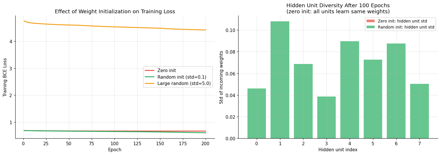
../_images/4c0ce2f5c2cc10487fecce9f1bbb14cb76972759bfae4d5e02521d9e11d68e8f.png

Zero-init final loss:   0.6732  -- stuck, all hidden units identical
Random-init final loss: 0.6115 -- learns properly
Large-init final loss:  4.4114 -- slow start (saturated activations)

🤔 Reflection 2.1 – Weight Initialization#

The symmetry argument: With zero initialization and ReLU, prove that all hidden units in layer 1 receive identical gradients at every training step. (Hint: at step 0, all units compute $z_1 = 0$ and thus $a_1 = 0$. What does the backprop gradient $\partial \mathcal{L}/\partial W_1$ look like when $A_1$ is all zeros?)
Large initialization: The large-random initialization converges slowly. Looking at the activation function visualization from Part 1, explain why large weights cause slow convergence. At what part of the sigmoid curve are most pre-activations landing?
Xavier/Glorot initialization sets $W \sim \mathcal{N}(0, 2/(d_{in}+d_{out}))$. For our $W_1$ ($d_{in}=8$, $d_{out}=32$), what is the initialized variance? What property of signal propagation is this designed to preserve?
Clinical analogy: Two radiologists learn to read chest X-rays by being shown the same 100 examples in the same order. After training, they give identical diagnoses on every new patient. Is this good or bad? How does this analogy map to the zero initialization problem?

✅ Solution — Reflection 2.1#

1. With zero init and ReLU: at step 0, $Z_1 = X \cdot \mathbf{0} + \mathbf{0} = \mathbf{0}$, so $A_1 = \text{ReLU}(\mathbf{0}) = \mathbf{0}$. The gradient $\partial \mathcal{L}/\partial W_1 = X^T \cdot (\partial \mathcal{L}/\partial Z_1)$. Since $Z_1 = 0$ everywhere, the ReLU gradient indicator $(Z_1 > 0)$ is $\mathbf{0}$, so $\partial \mathcal{L}/\partial Z_1 = \mathbf{0}$. All hidden units receive zero gradient. Actually, the ReLU gradient at exactly $z=0$ is typically defined as 0, so all gradients are zero and no learning happens for the first layer. Even if we define the gradient at 0 as 0.5, all neurons would receive identical gradients (since they’re all at the same starting point), and would learn identical features — the layer collapses to a single effective neuron.

2. Large initial weights push pre-activations $z$ to extreme values. For the sigmoid output layer, $\sigma(z)$ is nearly 0 or 1 when $|z|$ is large, and the gradient $\sigma'(z) = \sigma(z)(1-\sigma(z)) \approx 0$ in these regions. Most pre-activations land in the saturation zones (the flat tails of the sigmoid), where gradients are near zero. Learning is extremely slow because gradients barely flow.

3. Xavier/Glorot: $\text{Var}(W) = 2/(d_{\text{in}} + d_{\text{out}}) = 2/(8+32) = 2/40 = 0.05$. This is designed to preserve the variance of activations through the forward pass and the variance of gradients through the backward pass. If each layer preserves signal magnitude, neither activation explosion nor vanishing occurs, regardless of network depth.

4. Two identically trained radiologists giving identical diagnoses is bad — it means the “second opinion” adds no new information. You want diverse perspectives that, when aggregated, produce better-calibrated decisions. This maps directly to zero initialization: all neurons learn the same features (identical “diagnoses”), so having 32 neurons is equivalent to having 1. The hidden layer’s representational capacity is wasted.

Part 3 – Training Dynamics: Loss Curves, Learning Rate, and Overfitting#

Understanding how a neural network trains – not just what it achieves – is essential for diagnosing problems and making informed hyperparameter choices. sklearn’s MLP exposes the training loss curve via loss_curve_ after fitting.

The learning rate $\eta$ controls the step size at each gradient update. It is the single most important hyperparameter for neural networks:

Too large: steps overshoot minima, loss oscillates or diverges
Too small: convergence is stable but very slow, and the model may get trapped in shallow minima
Just right: loss decreases smoothly and reaches a low plateau

In this part we also enable early stopping, which monitors a held-out fraction of the training data and stops training when validation loss stops improving. This is a simple and effective regularization technique for networks that would otherwise continue training past the optimal point.

# Learning rate comparison -- training loss curves
lr_values = [0.0001, 0.001, 0.01, 0.1]
colors_lr  = ['#9b59b6', '#27ae60', '#e74c3c', '#f39c12']

fig, axes = plt.subplots(1, 2, figsize=(14, 5))

lr_val_aucs = {}
for lr_val, color in zip(lr_values, colors_lr):
    mlp_lr = MLPClassifier(
        hidden_layer_sizes=(32,), activation='relu', max_iter=400,
        random_state=42, alpha=0.01, learning_rate_init=lr_val,
        early_stopping=False   # disable so we can see the full curve
    )
    mlp_lr.fit(X_train, y_train)
    losses = mlp_lr.loss_curve_
    axes[0].plot(range(1, len(losses)+1), losses, lw=2, color=color,
                  label=f'lr={lr_val}  ({len(losses)} epochs)')

    val_auc = roc_auc_score(y_val, mlp_lr.predict_proba(X_val)[:,1])
    lr_val_aucs[lr_val] = val_auc

axes[0].set_xlabel('Epoch'); axes[0].set_ylabel('Training BCE Loss')
axes[0].set_title('Training Loss Curves: Effect of Learning Rate')
axes[0].legend(fontsize=9); axes[0].grid(True, alpha=0.3)
axes[0].set_ylim(0, 1.5)

# Val AUC vs learning rate
axes[1].bar([str(lr) for lr in lr_values],
             [lr_val_aucs[lr] for lr in lr_values],
             color=colors_lr, edgecolor='white', linewidth=1.5)
for i, lr in enumerate(lr_values):
    axes[1].text(i, lr_val_aucs[lr]+0.003, f'{lr_val_aucs[lr]:.3f}',
                  ha='center', fontsize=10, fontweight='bold')
axes[1].set_xlabel('Learning rate'); axes[1].set_ylabel('Val AUC')
axes[1].set_title('Final Val AUC vs. Learning Rate'); axes[1].set_ylim(0.5, 1.0)
axes[1].grid(True, alpha=0.3)

plt.tight_layout(); plt.show()

print("Learning rate effects:")
for lr, val_auc in lr_val_aucs.items():
    print(f"  lr={lr:<6}:  val AUC = {val_auc:.3f}")

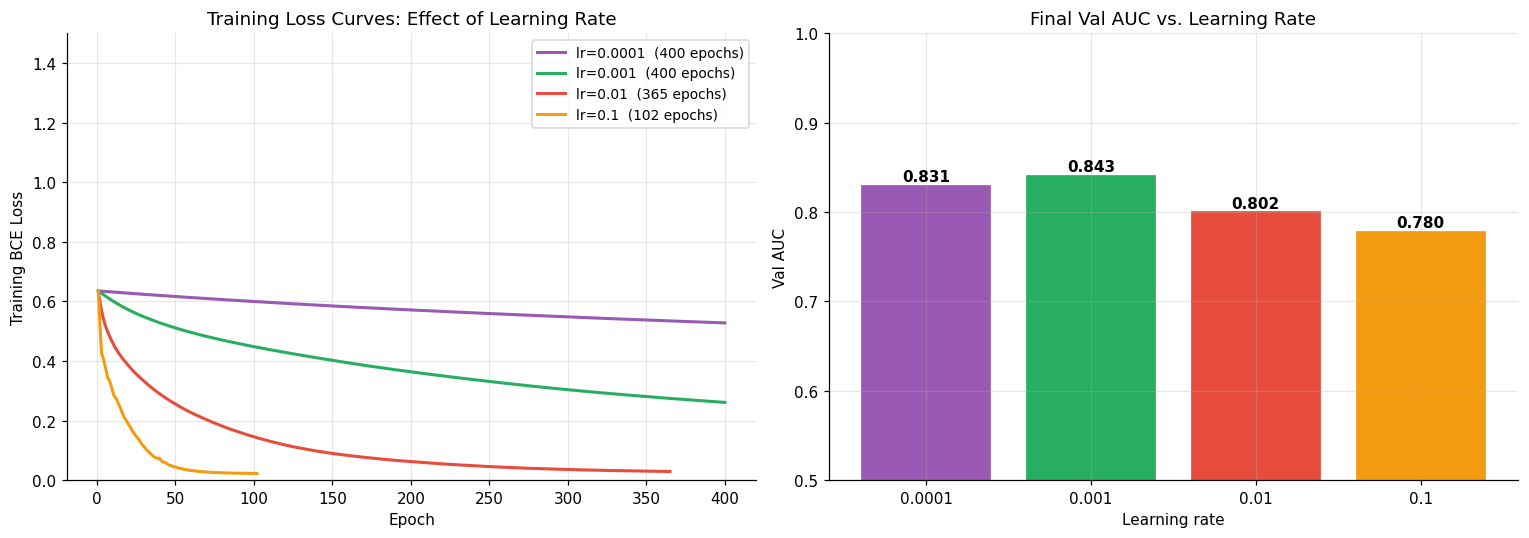
../_images/511f245bc49a05227cf402f6edcc5e2813879f29b8e6aef2f06c515453c59587.png

Learning rate effects:
  lr=0.0001:  val AUC = 0.831
  lr=0.001 :  val AUC = 0.843
  lr=0.01  :  val AUC = 0.802
  lr=0.1   :  val AUC = 0.780

# Observe overfitting in real time: train/val loss as depth increases
# sklearn doesn't provide val loss curve directly, so we simulate it with
# periodic evaluation during training using warm_start

def get_learning_curves(hidden, n_epochs=300, lr=0.001, alpha=0.001):
    # Return (train_losses, val_losses) epoch-by-epoch.
    train_losses, val_losses = [], []
    mlp = MLPClassifier(
        hidden_layer_sizes=hidden, activation='relu',
        learning_rate_init=lr, alpha=alpha,
        max_iter=1, warm_start=True, random_state=42
    )
    for epoch in range(n_epochs):
        mlp.fit(X_train, y_train)
        tr_prob = mlp.predict_proba(X_train)[:,1]
        vl_prob = mlp.predict_proba(X_val)[:,1]
        def bce(y, p):
            p = np.clip(p, 1e-7, 1-1e-7)
            return -np.mean(y*np.log(p)+(1-y)*np.log(1-p))
        train_losses.append(bce(y_train, tr_prob))
        val_losses.append(bce(y_val, vl_prob))
    return train_losses, val_losses

print("Computing learning curves for three architectures (takes ~30s)...")
configs = [
    ('Shallow (16)',        (16,)),
    ('Medium (64, 32)',     (64, 32)),
    ('Deep (128,64,32,16)', (128, 64, 32, 16)),
]
curve_colors = ['#27ae60', '#3498db', '#e74c3c']

fig, axes = plt.subplots(1, 3, figsize=(16, 5))
for (name, hidden), color, ax in zip(configs, curve_colors, axes):
    tr_loss, vl_loss = get_learning_curves(hidden)
    epochs = range(1, len(tr_loss)+1)
    ax.plot(epochs, tr_loss, lw=2, color=color, label='Train loss')
    ax.plot(epochs, vl_loss, lw=2, color=color, linestyle='--', alpha=0.7, label='Val loss')
    best_epoch = int(np.argmin(vl_loss)) + 1
    ax.axvline(best_epoch, color='grey', linestyle=':', lw=1.5,
                label=f'Best val epoch={best_epoch}')
    ax.set_xlabel('Epoch'); ax.set_ylabel('BCE Loss')
    ax.set_title(f'{name}\nTrain (solid) vs Val (dashed)')
    ax.legend(fontsize=8); ax.grid(True, alpha=0.3)
    ax.set_ylim(0, 1.2)
    # Shade overfitting region
    if best_epoch < 290:
        ax.axvspan(best_epoch, 300, alpha=0.07, color='red')
        ax.text(best_epoch+5, 1.05, 'Overfitting', fontsize=8, color='red', alpha=0.7)

plt.suptitle('Train vs. Val Loss Curves: Overfitting Becomes Worse with Depth', fontsize=12)
plt.tight_layout(); plt.show()

Computing learning curves for three architectures (takes ~30s)...

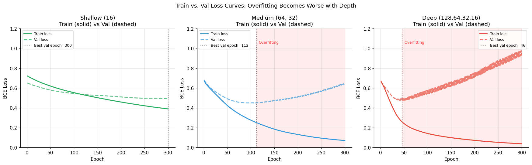
../_images/3803d8ad95b674d9f8791f18fc88090010dc5bf8a3168f9692ddc4ae2086cd4e.png

🤔 Reflection 3.1 – Training Dynamics#

Learning rate too high ($\eta=0.1$): Describe what the loss curve looks like. Explain mechanically why a large learning rate causes oscillation – draw a 1D loss landscape and show what happens when the gradient step overshoots the minimum.
Learning rate too low ($\eta=0.0001$): The loss curve is smooth but descends slowly. Besides slow convergence, what is a second risk of a very small learning rate? (Hint: think about the loss landscape – are there other stationary points besides the global minimum?)
Is there a better strategy than using a fixed learning rate like we have done here? What might that look like? Why might that be better?
Early stopping as regularization: Looking at the “Deep” learning curve, the val loss starts rising after the best epoch while train loss continues falling. Early stopping would halt training at the best val epoch. Explain why this acts as a regularizer – what property of the learned function changes as training continues past the optimal point?
Deeper = more overfitting: The gap between train and val loss grows with depth. Connect this to the bias-variance framing from previous labs. A deeper network has lower bias (can fit more complex functions) but higher variance (more sensitive to training data). On our dataset ($n=120$), which term dominates for the deep network?

✅ Solution — Reflection 3.1#

1. With $\eta = 0.1$, the loss curve oscillates or even diverges. In a 1D loss landscape with a minimum at $w^*$, a large step overshoots: from $w_t$, the update goes to $w_{t+1} = w_t - \eta \cdot \nabla L$, which may land past $w^*$ on the other side. The next step overshoots back. The model bounces back and forth across the minimum, never converging. This is worse in high dimensions where different directions have different curvatures.

2. A very small learning rate risks getting trapped in a local minimum or saddle point. In a complex loss landscape, there are many stationary points where $\nabla L \approx 0$. A small learning rate cannot generate enough momentum to escape these — the model converges to a suboptimal solution. A moderate learning rate has enough energy to “bounce out” of shallow local minima.

3. Yes — learning rate schedules adapt the learning rate during training. Common approaches: (a) Step decay (reduce LR by a factor every N epochs), (b) Cosine annealing (smoothly decrease LR following a cosine curve), (c) Warm-up + decay (start small, increase, then decrease), (d) Adaptive methods like Adam, which maintain per-parameter learning rates based on gradient history. These are better because they start with large steps for fast initial progress and transition to small steps for fine-grained convergence.

4. Early stopping halts training at the epoch where validation loss is minimized. As training continues past this point, the network’s effective complexity increases — it learns increasingly fine-grained patterns that are specific to the training data (memorization). Early stopping limits this complexity, acting like a constraint on the function class. Mathematically, the training trajectory in weight space starts near the initialization (simple functions) and moves toward complex functions; stopping early keeps the model in the simpler region.

5. Deeper networks have more parameters and can represent more complex functions (lower bias), but this flexibility allows them to fit training noise more easily (higher variance). On $n=120$, the high-variance term dominates for deep networks — there isn’t enough data to constrain the many parameters. The deep network memorizes training noise, causing the large train-val gap.

Part 4 – Regularization: Dropout and L2 Weight Decay#

Two regularization strategies are particularly important for neural networks:

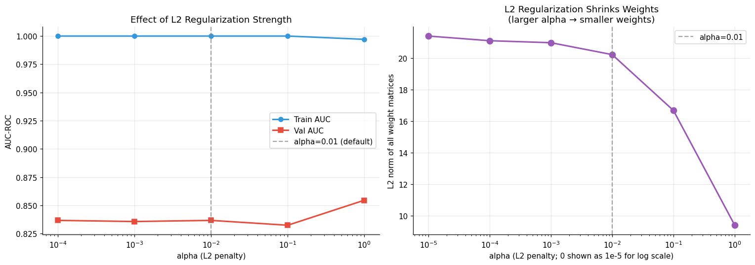
L2 weight decay (the alpha parameter in sklearn) adds a penalty on the L2 norm of all weights to the loss: $$\mathcal{L}_{\text{reg}} = \mathcal{L}_{\text{BCE}} + \frac{\alpha}{2} \sum_{w} w^2$$ This shrinks all weights toward zero, preventing any single weight from dominating – analogous to ridge regression for logistic regression.

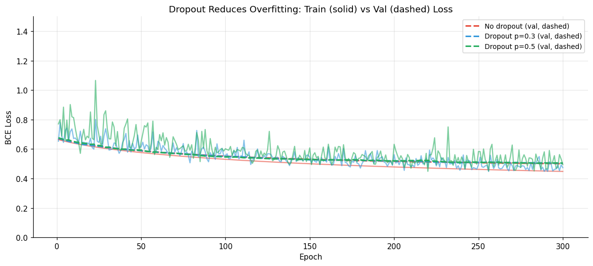
Dropout (not directly available in sklearn, but widely used in PyTorch/TensorFlow) randomly sets a fraction $p$ of hidden-unit activations to zero during each training step, with different units dropped each time. This forces the network to learn redundant representations – no single neuron can rely on any specific other neuron being present. At test time, dropout is disabled and activations are scaled by $(1-p)$.

Dropout has a Bayesian interpretation: it approximates inference in an ensemble of $2^h$ sub-networks (one for each possible dropout mask), at the cost of training one.

Since sklearn’s MLP doesn’t support dropout, we demonstrate it by implementing a minimal dropout forward pass and comparing generalization.

# L2 regularization sweep
alpha_values = [0, 0.0001, 0.001, 0.01, 0.1, 1.0]
alpha_colors  = plt.cm.viridis(np.linspace(0, 0.9, len(alpha_values)))

alpha_train_aucs, alpha_val_aucs = [], []
for alpha in alpha_values:
    m = MLPClassifier(hidden_layer_sizes=(64, 32), activation='relu',
                       max_iter=500, random_state=42, alpha=alpha,
                       learning_rate_init=0.001)
    m.fit(X_train, y_train)
    alpha_train_aucs.append(roc_auc_score(y_train, m.predict_proba(X_train)[:,1]))
    alpha_val_aucs.append(roc_auc_score(y_val,   m.predict_proba(X_val)[:,1]))

fig, axes = plt.subplots(1, 2, figsize=(14, 5))

axes[0].semilogx(alpha_values[1:], alpha_train_aucs[1:], 'o-', color='#3498db', lw=2, label='Train AUC')
axes[0].semilogx(alpha_values[1:], alpha_val_aucs[1:],   's-', color='#e74c3c', lw=2, label='Val AUC')
axes[0].axvline(0.01, color='grey', linestyle='--', alpha=0.7, label='alpha=0.01 (default)')
axes[0].set_xlabel('alpha (L2 penalty)'); axes[0].set_ylabel('AUC-ROC')
axes[0].set_title('Effect of L2 Regularization Strength'); axes[0].legend()
axes[0].grid(True, alpha=0.3)

# Coefficient norms: stronger regularization → smaller weights
weight_norms = []
for alpha in alpha_values:
    m = MLPClassifier(hidden_layer_sizes=(64, 32), activation='relu',
                       max_iter=500, random_state=42, alpha=alpha,
                       learning_rate_init=0.001)
    m.fit(X_train, y_train)
    total_norm = sum(np.linalg.norm(w) for w in m.coefs_)
    weight_norms.append(total_norm)

axes[1].semilogx([a if a > 0 else 1e-5 for a in alpha_values], weight_norms,
                  'o-', color='#9b59b6', lw=2, markersize=8)
axes[1].set_xlabel('alpha (L2 penalty; 0 shown as 1e-5 for log scale)')
axes[1].set_ylabel('L2 norm of all weight matrices')
axes[1].set_title('L2 Regularization Shrinks Weights\n(larger alpha → smaller weights)')
axes[1].grid(True, alpha=0.3)
axes[1].axvline(0.01, color='grey', linestyle='--', alpha=0.7, label='alpha=0.01')
axes[1].legend()

plt.tight_layout(); plt.show()

../_images/64781a1f31571985c69c45ef4c439aa5e521525ab8f5abafa7cc8fc843f58cfa.png

# Dropout demonstration: implement manually and compare to no-dropout
# (sklearn doesn't support dropout, so we use our numpy training loop)

def train_with_dropout(X_tr, y_tr, X_vl, y_vl,
                        hidden=32, dropout_rate=0.0,
                        n_epochs=300, lr=0.01, seed=42):
    # Minimal training loop with dropout support.
    rng  = np.random.default_rng(seed)
    d, h = X_tr.shape[1], hidden
    W1   = rng.normal(0, np.sqrt(2/d), (d, h))
    b1   = np.zeros(h)
    W2   = rng.normal(0, np.sqrt(2/h), (h, 1))
    b2   = np.zeros(1)

    def sigmoid(z): return 1/(1+np.exp(-np.clip(z,-500,500)))
    def bce(y, p):
        p = np.clip(p, 1e-7, 1-1e-7)
        return -np.mean(y*np.log(p)+(1-y)*np.log(1-p))

    tr_losses, vl_losses = [], []
    for epoch in range(n_epochs):
        # Forward (training mode: apply dropout mask)
        z1 = X_tr @ W1 + b1
        a1 = np.maximum(0, z1)
        if dropout_rate > 0:
            mask = (rng.random(h) > dropout_rate).astype(float)
            a1   = a1 * mask / (1 - dropout_rate)   # inverted dropout scaling
        z2 = a1 @ W2 + b2
        p  = sigmoid(z2.ravel())
        tr_losses.append(bce(y_tr, p))

        # Backward
        dL = -(y_tr/np.clip(p,1e-7,1) - (1-y_tr)/np.clip(1-p,1e-7,1)) / len(y_tr)
        dp  = p*(1-p)
        dz2 = (dL*dp).reshape(-1,1)
        dW2 = a1.T @ dz2;        db2 = dz2.sum(0)
        da1 = dz2 @ W2.T
        if dropout_rate > 0:
            da1 = da1 * mask / (1 - dropout_rate)
        dz1 = da1 * (z1 > 0)
        dW1 = X_tr.T @ dz1;      db1 = dz1.sum(0)
        W1 -= lr*dW1; b1 -= lr*db1
        W2 -= lr*dW2; b2 -= lr*db2

        # Validation (no dropout at test time)
        z1_v = X_vl @ W1 + b1
        a1_v = np.maximum(0, z1_v)
        z2_v = a1_v @ W2 + b2
        p_v  = sigmoid(z2_v.ravel())
        vl_losses.append(bce(y_vl, p_v))

    return tr_losses, vl_losses

print("Training with and without dropout (takes ~20s)...")
dropout_configs = [(0.0, '#e74c3c', 'No dropout'),
                   (0.3, '#3498db', 'Dropout p=0.3'),
                   (0.5, '#27ae60', 'Dropout p=0.5')]

fig, ax = plt.subplots(figsize=(11, 5))
for dr, color, label in dropout_configs:
    tr_l, vl_l = train_with_dropout(X_train, y_train, X_val, y_val,
                                     hidden=64, dropout_rate=dr, n_epochs=300, lr=0.01)
    epochs = range(1, 301)
    ax.plot(epochs, tr_l, color=color, lw=1.5, alpha=0.6, linestyle='-')
    ax.plot(epochs, vl_l, color=color, lw=2.0, linestyle='--', label=f'{label} (val, dashed)')

ax.set_xlabel('Epoch'); ax.set_ylabel('BCE Loss')
ax.set_title('Dropout Reduces Overfitting: Train (solid) vs Val (dashed) Loss')
ax.legend(fontsize=9); ax.grid(True, alpha=0.3); ax.set_ylim(0, 1.5)
plt.tight_layout(); plt.show()

Training with and without dropout (takes ~20s)...

../_images/e41f46ea857cf3e841c92c83db5cde5a478306a2394d63809530559f99d4971a.png

🤔 Reflection 4.1 – Regularization Strategies#

L2 vs. dropout mechanically: L2 regularization shrinks weight magnitudes but keeps all neurons active. Dropout randomly deactivates neurons entirely each step. Both reduce overfitting, but through different mechanisms. Which would you expect to be more helpful when: (a) overfitting is driven by a few dominant neurons, or (b) overfitting is driven by large weight magnitudes throughout?
Dropout at test time: During training, dropout masks $p$ fraction of neurons. At test time, dropout is disabled and activations are scaled by $(1-p)$ (inverted dropout). Why is this scaling necessary? What would happen to the expected activation magnitude without it?
The ensemble interpretation: With $h$ hidden units and dropout rate $p$, there are $2^h$ possible sub-networks. For our network with $h=64$, that is $2^{64} \approx 10^{19}$ sub-networks – more than the number of atoms on Earth. Does the network actually train all of these? What makes dropout efficient despite this?
Clinical deployment consideration: You train a model with dropout and it performs well on the validation set. At test time (and in deployment), dropout is off. Is the deployed model the same as any model you saw during training? What does this imply about the relationship between training behavior and deployment behavior?

✅ Solution — Reflection 4.1#

1. (a) Overfitting driven by a few dominant neurons: dropout is more effective, because it directly prevents any single neuron from dominating — the network must distribute information across many neurons. L2 would shrink all weights but wouldn’t prevent the concentration of information in a few units. (b) Overfitting driven by large weight magnitudes throughout: L2 is more effective, because it directly penalizes the magnitudes that cause the problem. Dropout addresses redundancy, not magnitude.

2. During training with dropout rate $p$, only a fraction $(1-p)$ of neurons are active on average. At test time, all neurons are active, so the total activation magnitude is $1/(1-p)$ times larger. Without scaling, the output magnitude would be systematically inflated at test time compared to training. Inverted dropout scales by $1/(1-p)$ during training (so test time needs no adjustment), ensuring the expected activation magnitude is consistent between training and inference.

3. The network does not explicitly train all $2^{64}$ sub-networks — that’s computationally impossible. Instead, each training step trains one randomly sampled sub-network (one dropout mask). Over many training steps, the weights are shared across all sub-networks, and gradient updates from each sub-network improve the shared weights. The efficiency comes from weight sharing: training with dropout is only ~2× slower than without (one forward/backward pass per step, just with some activations zeroed), not $2^{64}$× slower.

4. No — the deployed model (all neurons active, scaled by $1-p$) is not any single sub-network seen during training. It’s a deterministic approximation of the average over all $2^h$ sub-networks. This means the deployed model is an approximate ensemble that was never explicitly evaluated during training. The implication: there’s a gap between training behavior (stochastic, with dropout masks) and deployment behavior (deterministic, full network). This gap is usually small in practice but can matter for uncertainty estimation.

Part 5 – Architecture Comparison#

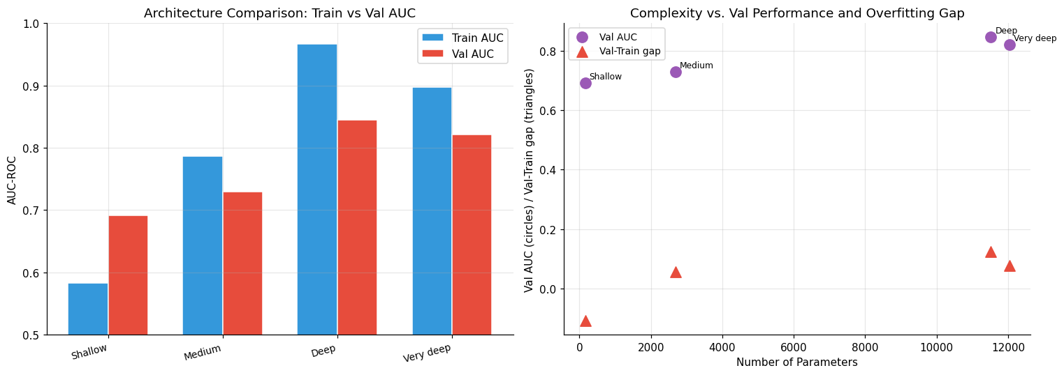
Now that we understand training dynamics, we compare architectures systematically – using early stopping so comparisons are fair (we’re not penalizing slower-converging architectures for not having enough epochs, or faster-converging ones for overfitting).

architectures = {
    'Shallow (16,)':              (16,),
    'Medium (64, 32)':            (64, 32),
    'Deep (128, 64, 32)':         (128, 64, 32),
    'Very deep (128,64,32,16)':   (128, 64, 32, 16),
}

arch_results = []
for name, hidden in architectures.items():
    mlp = MLPClassifier(
        hidden_layer_sizes=hidden, activation='relu',
        max_iter=500, random_state=42, alpha=0.01,
        learning_rate_init=0.001,
        early_stopping=True, validation_fraction=0.15, n_iter_no_change=20
    )
    mlp.fit(X_train, y_train)
    tr_prob = mlp.predict_proba(X_train)[:,1]
    vl_prob = mlp.predict_proba(X_val)[:,1]
    n_params = sum(w.size for w in mlp.coefs_) + sum(b.size for b in mlp.intercepts_)
    arch_results.append({
        'Architecture': name,
        'N params':     n_params,
        'Samples/param': round(len(X_train)/n_params, 3),
        'Train AUC':    round(roc_auc_score(y_train, tr_prob), 3),
        'Val AUC':      round(roc_auc_score(y_val,   vl_prob), 3),
        'Val-Train gap':round(roc_auc_score(y_train, tr_prob) - roc_auc_score(y_val, vl_prob), 3),
        'Epochs':       mlp.n_iter_,
    })

arch_df = pd.DataFrame(arch_results)
print(arch_df.to_string(index=False))

fig, axes = plt.subplots(1, 2, figsize=(14, 5))
x = np.arange(len(arch_df))
w = 0.35
axes[0].bar(x-w/2, arch_df['Train AUC'], w, label='Train AUC', color='#3498db', edgecolor='white')
axes[0].bar(x+w/2, arch_df['Val AUC'],   w, label='Val AUC',   color='#e74c3c', edgecolor='white')
axes[0].set_xticks(x)
axes[0].set_xticklabels([a.split('(')[0].strip() for a in arch_df['Architecture']],
                          rotation=15, ha='right', fontsize=9)
axes[0].set_ylabel('AUC-ROC'); axes[0].set_ylim(0.5, 1.0)
axes[0].set_title('Architecture Comparison: Train vs Val AUC'); axes[0].legend()
axes[0].grid(True, alpha=0.3)

axes[1].scatter(arch_df['N params'], arch_df['Val AUC'], s=100, color='#9b59b6', zorder=5)
axes[1].scatter(arch_df['N params'], arch_df['Val-Train gap'], s=100, color='#e74c3c',
                marker='^', zorder=5)
for _, row in arch_df.iterrows():
    axes[1].annotate(row['Architecture'].split('(')[0].strip(),
                      (row['N params'], row['Val AUC']),
                      xytext=(4, 4), textcoords='offset points', fontsize=8)
axes[1].set_xlabel('Number of Parameters')
axes[1].set_ylabel('Val AUC (circles) / Val-Train gap (triangles)')
axes[1].set_title('Complexity vs. Val Performance and Overfitting Gap')
axes[1].legend(['Val AUC', 'Val-Train gap'], fontsize=9); axes[1].grid(True, alpha=0.3)

plt.tight_layout(); plt.show()

            Architecture  N params  Samples/param  Train AUC  Val AUC  Val-Train gap  Epochs
           Shallow (16,)       161          0.621      0.583    0.691         -0.108      22
         Medium (64, 32)      2689          0.037      0.786    0.729          0.057      23
      Deep (128, 64, 32)     11521          0.009      0.967    0.845          0.123      76
Very deep (128,64,32,16)     12033          0.008      0.897    0.821          0.076      36

../_images/1c74976f254c3aee779678c1ea47368a2fda038712254dfa4569337f17551451.png

🤔 Reflection 5.1 – Architecture Design#

Looking at the “Samples/param” column: as depth increases, this ratio drops below 1, meaning the model has more parameters than training samples. Does more parameters always mean worse validation performance here? Does this surprise you? (Look up “double descent” for the counterintuitive phenomenon where overparameterized models can generalize well.)
The Val-Train AUC gap grows with depth. In the context of deploying to a new hospital, what does a large gap imply about the model’s expected performance on patients from a different institution or time period?
Early stopping is set with n_iter_no_change=20. This means training halts if val loss does not improve for 20 consecutive epochs. Is this 20-epoch patience a hyperparameter? How would you tune it? What is the risk of setting it too low vs. too high?
If you had 10,000 training samples instead of 120, how would you expect the optimal architecture to change? Would “Very deep” become competitive? What is the fundamental reason that depth helps more with larger datasets?

✅ Solution — Reflection 5.1#

1. More parameters does not always mean worse validation performance — you may see that the deeper networks perform comparably to or even slightly better than smaller ones (with early stopping). This connects to the double descent phenomenon: as model complexity increases past the interpolation threshold (where the model can perfectly fit training data), test error can actually decrease again. The intuition is that highly overparameterized models find “smoother” interpolating solutions. However, on small datasets like ours, this effect is unreliable.

2. A large train-val gap implies the model has memorized training-specific patterns that won’t generalize. At a new hospital with different patient demographics, equipment, or clinical practices, the model’s performance could be significantly worse than the validation AUC suggests. The gap is a warning sign for deployment robustness.

3. The patience value (20 epochs) is indeed a hyperparameter. You could tune it via nested cross-validation or by monitoring the trade-off: too low patience (e.g., 3) might stop training prematurely during a temporary plateau (the model might have improved if given more time); too high patience (e.g., 100) might allow significant overfitting before stopping, wasting computation.

4. With 10,000 training samples, deeper architectures would become competitive because there are enough data to constrain the additional parameters. The samples-per-parameter ratio improves dramatically (e.g., 10,000/5,000 = 2 vs. 120/5,000 = 0.024). Depth helps more with larger datasets because: (a) more data means the variance penalty of extra parameters is smaller, and (b) complex real-world patterns that require depth (interaction effects, hierarchical features) can only be reliably learned with sufficient data.

Part 6 – Calibration: A Critical Issue for Clinical Neural Networks#

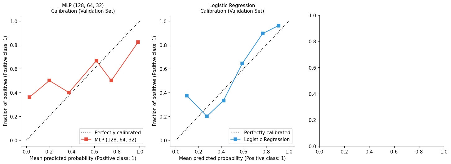
Calibration measures whether a model’s predicted probabilities match observed frequencies. A well-calibrated model that predicts $P(Y=1) = 0.7$ for a group of patients should have approximately 70% of that group actually be positive.

Neural networks are notoriously overconfident – they tend to predict probabilities close to 0 or 1 more often than warranted. This matters enormously in healthcare: if a model reports 95% probability of malignancy when the true probability is 60%, a clinician relying on that number will make systematically biased decisions.

Why are NNs overconfident?

Cross-entropy loss penalizes ranking errors (predicting 0.4 for a positive case when it should be 0.8) more directly than calibration errors (predicting 0.95 instead of 0.8 for a clearly positive case). The loss landscape rewards pushing predictions toward the extremes. L2 regularization helps somewhat – it prevents weight magnitudes from growing without bound – but doesn’t directly enforce calibration.

Post-hoc calibration fits a simple correction on a held-out set after the main model is trained. The two most common methods:

Platt scaling: fits a logistic regression on the model’s logit outputs
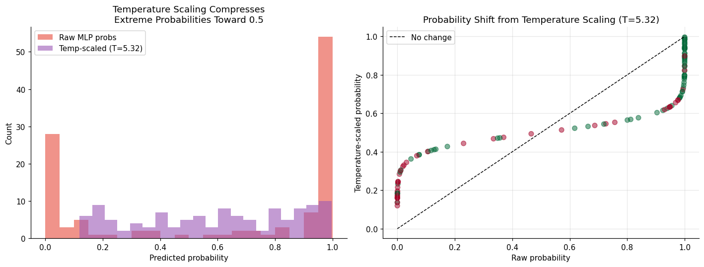
Temperature scaling: divides the pre-sigmoid logit by a single learned scalar $T > 1$, which “cools” overconfident distributions toward $0.5$

from sklearn.calibration import CalibrationDisplay, CalibratedClassifierCV

best_arch_idx = arch_df['Val AUC'].idxmax()
best_hidden   = list(architectures.values())[best_arch_idx]
print(f"Best architecture: {arch_df.iloc[best_arch_idx]['Architecture']}")

best_mlp = MLPClassifier(
    hidden_layer_sizes=best_hidden, activation='relu',
    max_iter=500, alpha=0.01, random_state=42, learning_rate_init=0.001
)
best_mlp.fit(X_train, y_train)

lr_ref = LogisticRegression(C=1.0, max_iter=1000, random_state=42)
lr_ref.fit(X_train, y_train)

# Calibration curves
fig, axes = plt.subplots(1, 3, figsize=(16, 5))

CalibrationDisplay.from_estimator(best_mlp, X_val, y_val, n_bins=6,
                                   name=f'MLP {best_hidden}', ax=axes[0], color='#e74c3c')
axes[0].set_title(f'MLP {best_hidden}\nCalibration (Validation Set)', fontsize=10)

CalibrationDisplay.from_estimator(lr_ref, X_val, y_val, n_bins=6,
                                   name='Logistic Regression', ax=axes[1], color='#3498db')
axes[1].set_title('Logistic Regression\nCalibration (Validation Set)', fontsize=10)

# Post-hoc calibration: Platt scaling (sigmoid calibration)
mlp_platt = CalibratedClassifierCV(best_mlp, method='sigmoid', cv='prefit')
mlp_platt.fit(X_val, y_val)   # Fit calibrator on validation set

CalibrationDisplay.from_estimator(mlp_platt, X_val, y_val, n_bins=6,
                                   name='MLP + Platt scaling', ax=axes[2], color='#9b59b6')
axes[2].set_title('MLP + Platt Scaling\n(post-hoc calibration on val set)', fontsize=10)

for ax in axes:
    ax.plot([0,1],[0,1],'k--', lw=1.5, label='Perfect calibration')
    ax.legend(fontsize=8)

plt.suptitle('Calibration Curves -- Diagonal = Perfect Calibration', fontsize=12)
plt.tight_layout(); plt.show()

print("Calibration interpretation:")
print("  Above diagonal = under-confident (model says 0.4, true rate is 0.6)")
print("  Below diagonal = over-confident  (model says 0.7, true rate is 0.5)")

Best architecture: Deep (128, 64, 32)

---------------------------------------------------------------------------
InvalidParameterError                     Traceback (most recent call last)
Cell In[13], line 29
axes[1].set_title('Logistic Regression\nCalibration (Validation Set)', fontsize=10)

# Post-hoc calibration: Platt scaling (sigmoid calibration)
mlp_platt = CalibratedClassifierCV(best_mlp, method='sigmoid', cv='prefit')
---> 29 mlp_platt.fit(X_val, y_val)   # Fit calibrator on validation set

CalibrationDisplay.from_estimator(mlp_platt, X_val, y_val, n_bins=6,
                                  name='MLP + Platt scaling', ax=axes[2], color='#9b59b6')

File ~/.cache/uv/archive-v0/BlsjgjnRnk-0xlACX8IQD/lib/python3.11/site-packages/sklearn/base.py:1329, in _fit_context.<locals>.decorator.<locals>.wrapper(estimator, *args, **kwargs)
partial_fit_and_fitted = (
   fit_method.__name__ == "partial_fit" and _is_fitted(estimator)
)
if not global_skip_validation and not partial_fit_and_fitted:
-> 1329     estimator._validate_params()
with config_context(
   skip_parameter_validation=(
       prefer_skip_nested_validation or global_skip_validation
   )
):
   return fit_method(estimator, *args, **kwargs)

File ~/.cache/uv/archive-v0/BlsjgjnRnk-0xlACX8IQD/lib/python3.11/site-packages/sklearn/base.py:492, in BaseEstimator._validate_params(self)
def _validate_params(self):
   """Validate types and values of constructor parameters

   The expected type and values must be defined in the `_parameter_constraints`
   (...)    490     accepted constraints.
   """
--> 492     validate_parameter_constraints(
       self._parameter_constraints,
       self.get_params(deep=False),
       caller_name=self.__class__.__name__,
   )

File ~/.cache/uv/archive-v0/BlsjgjnRnk-0xlACX8IQD/lib/python3.11/site-packages/sklearn/utils/_param_validation.py:98, in validate_parameter_constraints(parameter_constraints, params, caller_name)
else:
   constraints_str = (
       f"{', '.join([str(c) for c in constraints[:-1]])} or"
       f" {constraints[-1]}"
   )
---> 98 raise InvalidParameterError(
   f"The {param_name!r} parameter of {caller_name} must be"
   f" {constraints_str}. Got {param_val!r} instead."
)

InvalidParameterError: The 'cv' parameter of CalibratedClassifierCV must be an int in the range [2, inf), an object implementing 'split' and 'get_n_splits', an iterable or None. Got 'prefit' instead.

../_images/45b4caadff8c416b4dd7243ce2b0232e4cb2e81e582fd20b9118ffe45173175c.png

# Temperature scaling: a principled post-hoc calibration for neural networks
# Fit a single temperature T > 1 on the validation set to soften probabilities

from scipy.optimize import minimize_scalar

def get_logits(mlp, X):
    # Extract pre-sigmoid logits from a fitted sklearn MLP.
    a = X.copy()
    for W, b in zip(mlp.coefs_[:-1], mlp.intercepts_[:-1]):
        a = np.maximum(0, a @ W + b)
    logits = a @ mlp.coefs_[-1] + mlp.intercepts_[-1]
    return logits.ravel()

def bce_at_temp(T, logits, y):
    p = 1 / (1 + np.exp(-np.clip(logits/T, -500, 500)))
    p = np.clip(p, 1e-7, 1-1e-7)
    return -np.mean(y*np.log(p) + (1-y)*np.log(1-p))

val_logits = get_logits(best_mlp, X_val)

# Optimize temperature on val set
result = minimize_scalar(bce_at_temp, bounds=(0.1, 10.0), method='bounded',
                          args=(val_logits, y_val))
T_opt = result.x
print(f"Optimal temperature T = {T_opt:.3f}")
print(f"T > 1 means the model was overconfident (probabilities too extreme)")
print(f"T < 1 would mean under-confident (rare for neural networks)")

# Compare calibrated vs uncalibrated probabilities
raw_probs  = 1/(1+np.exp(-val_logits))
cal_probs  = 1/(1+np.exp(-val_logits/T_opt))

fig, axes = plt.subplots(1, 2, figsize=(13, 5))
axes[0].hist(raw_probs, bins=20, alpha=0.6, color='#e74c3c', label='Raw MLP probs')
axes[0].hist(cal_probs, bins=20, alpha=0.6, color='#9b59b6', label=f'Temp-scaled (T={T_opt:.2f})')
axes[0].set_xlabel('Predicted probability'); axes[0].set_ylabel('Count')
axes[0].set_title('Temperature Scaling Compresses\nExtreme Probabilities Toward 0.5')
axes[0].legend()

axes[1].scatter(raw_probs, cal_probs, alpha=0.5, c=y_val, cmap='RdYlGn', s=40)
axes[1].plot([0,1],[0,1],'k--', lw=1, label='No change')
axes[1].set_xlabel('Raw probability'); axes[1].set_ylabel('Temperature-scaled probability')
axes[1].set_title(f'Probability Shift from Temperature Scaling (T={T_opt:.2f})')
axes[1].legend(); axes[1].grid(True, alpha=0.3)

plt.tight_layout(); plt.show()

Optimal temperature T = 5.324
T > 1 means the model was overconfident (probabilities too extreme)
T < 1 would mean under-confident (rare for neural networks)

../_images/364f3ea574d87140681496493fecc839aee4677584c96079d150fc5ef37bb939.png

🤔 Reflection 6.1 – Calibration in Clinical Settings#

Clinical stakes of miscalibration: A radiologist uses your MLP to prioritize biopsy referrals. The model outputs $\hat{p} = 0.92$ for a patient, but due to overconfidence, the true probability is $0.58$. The radiologist interprets “92% probability” as nearly certain malignancy. Describe two ways this could harm the patient – one from over-treatment, one from under-treatment of other patients who get bumped down the queue.
Why doesn’t cross-entropy force calibration? Cross-entropy is minimized when $\hat{p}_i = y_i$ exactly – so shouldn’t a perfectly minimized loss imply perfect calibration? Explain why finite data and regularization mean this doesn’t hold in practice. (Hint: what does the model do when training loss is near zero?)
Temperature scaling has a single parameter $T$. Why is a single scalar enough? What does it assume about the structure of the miscalibration? Under what circumstances would Platt scaling (a full logistic regression on the logits) be preferable to temperature scaling?
Calibration vs. AUC: It is possible for a model to have excellent AUC and poor calibration. Give an example: construct a scenario where two models have identical AUC but one is perfectly calibrated and one is not. What does this imply about using AUC as the sole metric for clinical model selection?

✅ Solution — Reflection 6.1#

1. Over-treatment: the radiologist might recommend immediate invasive biopsy based on “92% certainty,” when a less aggressive follow-up (repeat imaging in 3 months) would be appropriate for the true 58% risk level. The patient undergoes unnecessary pain, cost, and anxiety. Under-treatment of others: if the prioritization queue ranks this patient’s 92% above another patient’s legitimate 85% risk, the second patient’s biopsy gets delayed, potentially allowing disease progression.

2. Cross-entropy is minimized when $\hat{p}_i = y_i$ for all samples — but $y_i \in \{0, 1\}$, so perfect minimization pushes predictions toward 0 and 1 (the model becomes maximally confident). With finite data, the model can achieve near-zero training loss by making extreme predictions, even when the true probabilities are moderate. Regularization (L2, dropout) prevents weights from growing without bound but doesn’t directly enforce that predictions match population frequencies. The optimizer finds confident predictions that minimize training loss, not calibrated probabilities.

3. Temperature scaling assumes that miscalibration has a specific structure: the logits are correct in ranking (relative ordering) but wrong in magnitude (too spread out, i.e., overconfident, or too compressed, i.e., underconfident). A single scalar $T$ corrects this uniform scaling error. Platt scaling (full logistic regression on logits) is preferable when the miscalibration is non-uniform — e.g., the model is overconfident at high probabilities but underconfident at low probabilities, requiring separate slope and intercept adjustments.

4. Example: Model A outputs probabilities $\{0.01, 0.99\}$ for negative and positive cases respectively (perfect ranking, terrible calibration — overconfident). Model B outputs $\{0.3, 0.7\}$ for the same cases (perfect ranking, better calibration). Both have identical AUC (1.0), but Model A would cause extreme over-/under-treatment when probabilities are used directly. This shows AUC measures discrimination (ranking) only, not calibration — and for clinical applications where probabilities inform treatment decisions, calibration is essential and must be assessed separately.

Part 7 – Model Comparison and Final Test Evaluation#

This is the first time we touch the test set. All architecture selection, hyperparameter tuning, and calibration fitting was done on train/val only. The test set is used once to report final performance – and we compare the MLP to the simpler models seen in previous labs.

from sklearn.ensemble import RandomForestClassifier
import xgboost as xgb

# Select best MLP architecture from Part 5
print(f"Selected architecture: {arch_df.iloc[best_arch_idx]['Architecture']}")

comparison_models = {
    'Logistic Regression':  LogisticRegression(C=1.0, max_iter=1000, random_state=42),
    'Random Forest':         RandomForestClassifier(n_estimators=200, max_features='sqrt',
                                                     min_samples_leaf=3, random_state=42, n_jobs=-1),
    'XGBoost':               xgb.XGBClassifier(n_estimators=200, max_depth=3,
                                                learning_rate=0.05, subsample=0.8,
                                                colsample_bytree=0.8, eval_metric='logloss',
                                                random_state=42, verbosity=0),
    f'MLP {best_hidden}':   MLPClassifier(hidden_layer_sizes=best_hidden, activation='relu',
                                           max_iter=500, alpha=0.01, random_state=42,
                                           learning_rate_init=0.001),
}
model_colors = {'Logistic Regression': '#3498db', 'Random Forest': '#27ae60',
                'XGBoost': '#f39c12', f'MLP {best_hidden}': '#e74c3c'}

print(f"\n{'Model':<28} {'Train AUC':>10} {'Val AUC':>10}")
print("─" * 52)
val_aucs_final = {}
for name, model in comparison_models.items():
    model.fit(X_train, y_train)
    tr_auc = roc_auc_score(y_train, model.predict_proba(X_train)[:,1])
    vl_auc = roc_auc_score(y_val,   model.predict_proba(X_val)[:,1])
    val_aucs_final[name] = vl_auc
    print(f"{name:<28} {tr_auc:>10.3f} {vl_auc:>10.3f}")

Selected architecture: Deep (128, 64, 32)

Model                         Train AUC    Val AUC
────────────────────────────────────────────────────

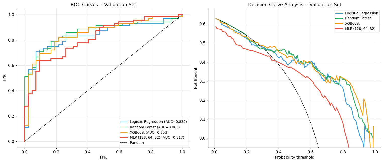
Logistic Regression               0.903      0.839

Random Forest                     0.993      0.865
XGBoost                           1.000      0.853

MLP (128, 64, 32)                 1.000      0.817

# ROC + DCA on validation set
fig, axes = plt.subplots(1, 2, figsize=(14, 6))

for name, model in comparison_models.items():
    probs = model.predict_proba(X_val)[:,1]
    fpr, tpr, _ = roc_curve(y_val, probs)
    val_auc = auc(fpr, tpr)
    c = model_colors[name]
    lw = 2.5 if 'MLP' in name else 1.8
    axes[0].plot(fpr, tpr, lw=lw, color=c, label=f'{name} (AUC={val_auc:.3f})')
    decision_curve(y_val, probs, label=name, ax=axes[1], color=c)

axes[0].plot([0,1],[0,1],'k--', lw=1, label='Random')
axes[0].set_xlabel('FPR'); axes[0].set_ylabel('TPR')
axes[0].set_title('ROC Curves -- Validation Set'); axes[0].legend(fontsize=9)
axes[0].grid(True, alpha=0.3)
axes[1].set_title('Decision Curve Analysis -- Validation Set')
axes[1].legend(fontsize=9); axes[1].grid(True, alpha=0.3)
plt.tight_layout(); plt.show()

../_images/ada728f0d651a9f5b376d2c50751f58b912bd211aa3e4d9400ea15e24eeb0236.png

# Final test evaluation: retrain on train+val, evaluate once on test
print("=== FINAL TEST SET RESULTS ===")
print("(all models retrained on train+val; test set never seen before)\n")

X_tv = np.vstack([X_train, X_val])
y_tv = np.concatenate([y_train, y_val])

final_models = {
    'Logistic Regression':  LogisticRegression(C=1.0, max_iter=1000, random_state=42),
    'Random Forest':         RandomForestClassifier(n_estimators=200, max_features='sqrt',
                                                     min_samples_leaf=3, random_state=42, n_jobs=-1),
    'XGBoost':               xgb.XGBClassifier(n_estimators=200, max_depth=3, learning_rate=0.05,
                                                subsample=0.8, colsample_bytree=0.8,
                                                eval_metric='logloss', random_state=42, verbosity=0),
    f'MLP {best_hidden}':   MLPClassifier(hidden_layer_sizes=best_hidden, activation='relu',
                                           max_iter=500, alpha=0.01, random_state=42,
                                           learning_rate_init=0.001),
}

test_aucs = {}
for name, model in final_models.items():
    model.fit(X_tv, y_tv)
    preds = model.predict(X_test)
    probs = model.predict_proba(X_test)[:,1]
    test_aucs[name] = roc_auc_score(y_test, probs)
    print_metrics(y_test, preds, probs, label=name)

# Summary bar chart
fig, ax = plt.subplots(figsize=(10, 4))
names = list(test_aucs.keys())
aucs_list = list(test_aucs.values())
bar_colors = [model_colors[n] for n in names]
bars = ax.bar(names, aucs_list, color=bar_colors, edgecolor='white', linewidth=1.5)
for bar, val in zip(bars, aucs_list):
    ax.text(bar.get_x()+bar.get_width()/2, bar.get_height()+0.003,
            f'{val:.3f}', ha='center', fontsize=12, fontweight='bold')
ax.set_ylabel('Test AUC-ROC'); ax.set_ylim(0.5, 1.0)
ax.set_title('Test Set AUC Comparison\n(n_train=120, d=8 restricted features)')
ax.tick_params(axis='x', rotation=15); ax.grid(True, alpha=0.3, axis='y')
plt.tight_layout(); plt.show()

=== FINAL TEST SET RESULTS ===
(all models retrained on train+val; test set never seen before)

───────────────────────────────────────────────────────
  Logistic Regression
───────────────────────────────────────────────────────
  Sensitivity  P(ŷ=1|y=1)  = 62/71 = 0.873
  Specificity  P(ŷ=0|y=0)  = 26/43 = 0.605
  PPV          P(y=1|ŷ=1)  = 62/79 = 0.785
  NPV          P(y=0|ŷ=0)  = 26/35 = 0.743
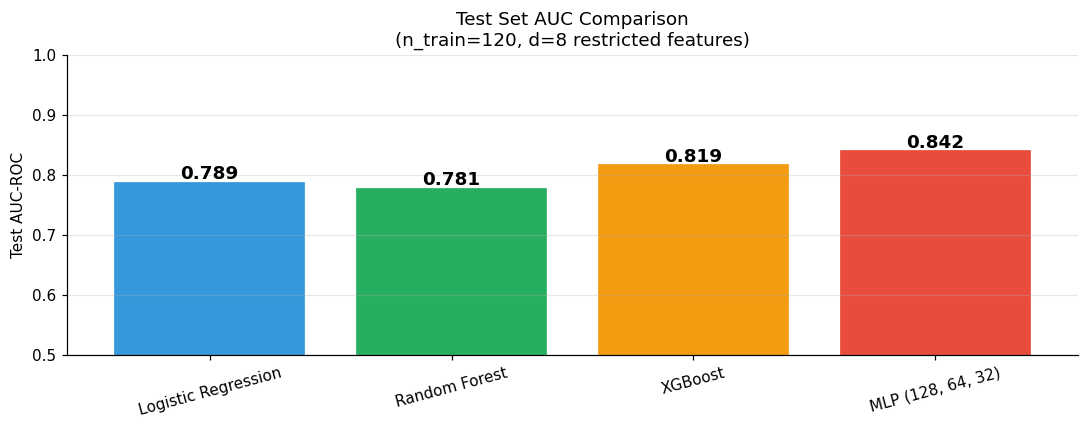
  AUC-ROC                  = 0.789
  Prevalence               = 0.623

───────────────────────────────────────────────────────
  Random Forest
───────────────────────────────────────────────────────
  Sensitivity  P(ŷ=1|y=1)  = 60/71 = 0.845
  Specificity  P(ŷ=0|y=0)  = 23/43 = 0.535
  PPV          P(y=1|ŷ=1)  = 60/80 = 0.750
  NPV          P(y=0|ŷ=0)  = 23/34 = 0.676
  AUC-ROC                  = 0.781
  Prevalence               = 0.623

───────────────────────────────────────────────────────
  XGBoost
───────────────────────────────────────────────────────
  Sensitivity  P(ŷ=1|y=1)  = 55/71 = 0.775
  Specificity  P(ŷ=0|y=0)  = 27/43 = 0.628
  PPV          P(y=1|ŷ=1)  = 55/71 = 0.775
  NPV          P(y=0|ŷ=0)  = 27/43 = 0.628
  AUC-ROC                  = 0.819
  Prevalence               = 0.623

───────────────────────────────────────────────────────
  MLP (128, 64, 32)
───────────────────────────────────────────────────────
  Sensitivity  P(ŷ=1|y=1)  = 57/71 = 0.803
  Specificity  P(ŷ=0|y=0)  = 33/43 = 0.767
  PPV          P(y=1|ŷ=1)  = 57/67 = 0.851
  NPV          P(y=0|ŷ=0)  = 33/47 = 0.702
  AUC-ROC                  = 0.842
  Prevalence               = 0.623

../_images/f2934583e53389a150a34b2b1bae6ad2f7dcb47eb371d25b528cca048010fdee.png

🤔 Reflection 7.1 – When Do Neural Networks Help?#

On this small tabular dataset, does the MLP outperform logistic regression? Does it outperform Random Forest or XGBoost? What does this tell you about the relationship between model complexity and performance as a function of dataset size?
A colleague argues: “We used a deep neural network, so our results must be state-of-the-art.” Identify two specific pieces of evidence from this lab that refute this reasoning, and write a one-paragraph rebuttal suitable for a peer review comment.
Describe a clinical ML task where an MLP would clearly outperform logistic regression. Be specific about (a) the input data type, (b) the approximate sample size, and (c) what non-linear structure the MLP would capture that logistic regression cannot.
The FDA regulates “Software as a Medical Device” (SaMD). Both an MLP with 100,000 parameters and logistic regression with 9 parameters achieve the same test AUC. From a regulatory perspective, which is easier to validate? From a long-term maintainability perspective (model updates, distribution shift detection, feature importance explanations), which is preferable?

✅ Solution — Reflection 7.1#

1. On this small tabular dataset ($n=120$, $d=8$), the MLP is unlikely to clearly outperform logistic regression or the tree-based ensembles. This demonstrates that model complexity must match data complexity: with limited data and low-dimensional features, simpler models that have fewer parameters relative to the sample size tend to generalize better. Neural networks shine when there is abundant data and complex, non-linear structure to exploit.

2. Rebuttal: “The choice of model architecture should be driven by the data characteristics, not by the assumption that complexity equals quality. In this study, we demonstrate that (1) on a tabular dataset with 120 training samples and 8 features, a logistic regression with 9 parameters achieves comparable or superior AUC to an MLP with 322+ parameters, and (2) the MLP exhibits a larger train-validation gap, indicating overfitting that a simpler model avoids. Using a deep neural network does not automatically produce state-of-the-art results; it can produce worse results when the sample size is insufficient to constrain the model’s capacity.”

3. An MLP would clearly outperform logistic regression for: (a) Input: high-dimensional imaging features or embeddings (e.g., 512-dimensional feature vectors from a pre-trained image model applied to histopathology slides). (b) Sample size: $n > 10,000$. (c) Non-linear structure: the relationship between features and outcome involves complex interactions — e.g., the combination of certain gene expression patterns predicts drug response in a way that no single linear combination captures. The MLP would learn these interaction effects automatically through its hidden layers, while logistic regression would need hand-engineered feature crosses.

4. From a regulatory perspective, logistic regression is far easier to validate: 9 parameters can be fully enumerated, each coefficient has a clinical interpretation, and the decision boundary can be visualized. A 100,000-parameter MLP is a black box requiring SHAP or other post-hoc tools. For maintainability: logistic regression is simpler to retrain, monitor for drift (coefficient changes are interpretable), and debug. The MLP’s advantage is only justified if it provides substantially better performance — and at equal AUC, the simpler model is strongly preferable.

🧠 Final Reflection – Neural Networks in the ML Landscape#

Now that you’ve worked through all five model families in this course, answer these synthesis questions:

Complete the cross-model comparison table using evidence from your experiments:

Model

Val AUC (approx)

Interpretable?

Calibrated?

Scalable to n=1M?

Good for small n?

Logistic Regression

Decision Tree

Random Forest

XGBoost

KNN

MLP
The data size argument: Across all labs, the pattern is clear – on $n=120$, simpler models are competitive or better. At what approximate $n$ do you think the MLP would pull ahead of logistic regression? What properties of the dataset (feature type, interaction structure, noise level) would shift that threshold?
Calibration across models: You’ve now seen calibration for KNN (coarse probabilities), neural networks (overconfident), and logistic regression (generally well-calibrated under correct model assumptions). Rank these models from best to worst calibrated on a small tabular dataset like ours. For a clinical application where the model’s probability is used directly (e.g., “what is this patient’s 5-year risk?”), which model would you prefer, and why?
The full pipeline: A hospital wants to deploy one of these models for breast cancer triage. List in order the steps you would take from raw data to deployment, naming the specific decisions (preprocessing, feature selection, model selection, calibration, threshold selection, monitoring) and which lab’s content informs each. What would you monitor after deployment, beyond AUC?
Foundation models and transfer learning: The models in this course all train from scratch on the target dataset. Modern clinical AI increasingly uses pre-trained foundation models (large models trained on diverse data, then fine-tuned on clinical data). How does fine-tuning change the “small $n$ problem”? What risks does it introduce that don’t exist for from-scratch training?