Neural Networks: From Motivation to Practice

BINF 4002 — Machine Learning for Health — Companion Lab

This notebook accompanies the lecture on neural networks. We’ll build intuition by:

1. Building a simple MLP from scratch and training it on MNIST

2. Visualizing what goes wrong with bad initialization

3. Comparing normalization strategies

4. Exploring learning rate and batch size interactions

5. Demonstrating gradient clipping and accumulation

6. Monitoring training with Weights & Biases

Run in Colab: Click Runtime → Run all or step through cell by cell.

---

0. Setup

# Install wandb if needed (Colab)
# (pip install handled by the book's isolated env)

import torch
import torch.nn as nn
import torch.optim as optim
from torch.utils.data import DataLoader
from torchvision import datasets, transforms
import matplotlib.pyplot as plt
import numpy as np
import copy
import warnings
warnings.filterwarnings('ignore')

# For reproducibility
torch.manual_seed(42)
np.random.seed(42)

device = torch.device('cuda' if torch.cuda.is_available() else 'cpu')
print(f"Using device: {device}")

/bin/bash: line 1: pip: command not found

Using device: cpu

# Load MNIST
transform = transforms.Compose([
    transforms.ToTensor(),
    transforms.Normalize((0.1307,), (0.3081,))  # MNIST mean and std
])

train_dataset = datasets.MNIST('./data', train=True, download=True, transform=transform)
test_dataset = datasets.MNIST('./data', train=False, transform=transform)

# We'll use a subset for faster experiments
train_subset = torch.utils.data.Subset(train_dataset, range(10000))
test_subset = torch.utils.data.Subset(test_dataset, range(2000))

print(f"Training samples: {len(train_subset)}")
print(f"Test samples: {len(test_subset)}")
print(f"Input shape: {train_dataset[0][0].shape} → flattened to {28*28}")
print(f"Number of classes: 10")

  0%|          | 0.00/9.91M [00:00<?, ?B/s]

  7%|▋         | 655k/9.91M [00:00<00:01, 6.50MB/s]

 47%|████▋     | 4.69M/9.91M [00:00<00:00, 25.9MB/s]

 92%|█████████▏| 9.11M/9.91M [00:00<00:00, 33.6MB/s]

100%|██████████| 9.91M/9.91M [00:00<00:00, 29.0MB/s]

  0%|          | 0.00/28.9k [00:00<?, ?B/s]

100%|██████████| 28.9k/28.9k [00:00<00:00, 2.64MB/s]

  0%|          | 0.00/1.65M [00:00<?, ?B/s]

 26%|██▌       | 426k/1.65M [00:00<00:00, 4.07MB/s]

100%|██████████| 1.65M/1.65M [00:00<00:00, 8.72MB/s]

  0%|          | 0.00/4.54k [00:00<?, ?B/s]

100%|██████████| 4.54k/4.54k [00:00<00:00, 5.13MB/s]

Training samples: 10000
Test samples: 2000
Input shape: torch.Size([1, 28, 28]) → flattened to 784
Number of classes: 10

# Visualize a few examples
fig, axes = plt.subplots(1, 8, figsize=(14, 2))
for i, ax in enumerate(axes):
    img, label = train_dataset[i]
    ax.imshow(img.squeeze(), cmap='gray')
    ax.set_title(f"Label: {label}")
    ax.axis('off')
plt.suptitle("MNIST Samples", fontsize=14)
plt.tight_layout()
plt.show()

---

1. The Core Building Block: act(Wx + b)

Let’s build an MLP from first principles before using nn.Sequential.

class ManualMLP(nn.Module):
    """MLP written explicitly to show what's happening inside."""

    def __init__(self, input_dim=784, hidden_dim=256, output_dim=10):
        super().__init__()
        # Layer 1: input → hidden
        self.W1 = nn.Parameter(torch.randn(hidden_dim, input_dim) * 0.01)
        self.b1 = nn.Parameter(torch.zeros(hidden_dim))

        # Layer 2: hidden → hidden
        self.W2 = nn.Parameter(torch.randn(hidden_dim, hidden_dim) * 0.01)
        self.b2 = nn.Parameter(torch.zeros(hidden_dim))

        # Layer 3: hidden → output
        self.W3 = nn.Parameter(torch.randn(output_dim, hidden_dim) * 0.01)
        self.b3 = nn.Parameter(torch.zeros(output_dim))

    def forward(self, x):
        # Flatten: (batch, 1, 28, 28) → (batch, 784)
        x = x.view(x.size(0), -1)

        # Layer 1: act(W1 @ x + b1)
        h1 = torch.relu(x @ self.W1.T + self.b1)

        # Layer 2: act(W2 @ h1 + b2)
        h2 = torch.relu(h1 @ self.W2.T + self.b2)

        # Layer 3: W3 @ h2 + b3 (no activation — logits for cross-entropy)
        logits = h2 @ self.W3.T + self.b3

        return logits

# Count parameters
model = ManualMLP()
n_params = sum(p.numel() for p in model.parameters())
print(f"Total parameters: {n_params:,}")
print(f"  W1: {784}×{256} = {784*256:,}")
print(f"  W2: {256}×{256} = {256*256:,}")
print(f"  W3: {256}×{10}  = {256*10:,}")
print(f"  biases: {256+256+10:,}")

Total parameters: 269,322
  W1: 784×256 = 200,704
  W2: 256×256 = 65,536
  W3: 256×10  = 2,560
  biases: 522

The same thing in idiomatic PyTorch (this is equivalent):

def make_mlp(hidden_dim=256, num_layers=3, use_batchnorm=False, use_layernorm=False,
             use_residual=False, dropout=0.0, activation='relu'):
    """Flexible MLP builder for our experiments."""

    act_fn = {'relu': nn.ReLU, 'gelu': nn.GELU, 'tanh': nn.Tanh, 'sigmoid': nn.Sigmoid}

    class FlexMLP(nn.Module):
        def __init__(self):
            super().__init__()
            layers = []
            dims = [784] + [hidden_dim] * (num_layers - 1) + [10]

            self.blocks = nn.ModuleList()
            self.use_residual = use_residual

            for i in range(len(dims) - 1):
                block = [nn.Linear(dims[i], dims[i+1])]

                if i < len(dims) - 2:  # No activation/norm on last layer
                    if use_batchnorm:
                        block.append(nn.BatchNorm1d(dims[i+1]))
                    if use_layernorm:
                        block.append(nn.LayerNorm(dims[i+1]))
                    block.append(act_fn[activation]())
                    if dropout > 0:
                        block.append(nn.Dropout(dropout))

                self.blocks.append(nn.Sequential(*block))

        def forward(self, x):
            x = x.view(x.size(0), -1)
            for i, block in enumerate(self.blocks):
                if self.use_residual and i > 0 and i < len(self.blocks) - 1:
                    x = x + block(x)  # Residual connection
                else:
                    x = block(x)
            return x

    return FlexMLP()

---

2. Training Utilities

Let’s write a flexible training loop we can reuse for all experiments.

def train_model(model, train_loader, test_loader, epochs=20, lr=1e-3,
                optimizer_type='adam', weight_decay=0, grad_clip=None,
                accumulation_steps=1, scheduler_type=None, warmup_epochs=0,
                use_wandb=False, run_name=None, verbose=True):
    """
    General training loop with all the bells and whistles.

    Returns: dict with training history
    """
    model = model.to(device)
    criterion = nn.CrossEntropyLoss()

    # Optimizer
    if optimizer_type == 'adam':
        optimizer = optim.Adam(model.parameters(), lr=lr, weight_decay=weight_decay)
    elif optimizer_type == 'adamw':
        optimizer = optim.AdamW(model.parameters(), lr=lr, weight_decay=weight_decay)
    elif optimizer_type == 'sgd':
        optimizer = optim.SGD(model.parameters(), lr=lr, momentum=0.9, weight_decay=weight_decay)

    # Scheduler
    scheduler = None
    if scheduler_type == 'cosine':
        scheduler = optim.lr_scheduler.CosineAnnealingLR(optimizer, T_max=epochs)
    elif scheduler_type == 'step':
        scheduler = optim.lr_scheduler.StepLR(optimizer, step_size=epochs//3, gamma=0.1)

    history = {
        'train_loss': [], 'test_loss': [],
        'train_acc': [], 'test_acc': [],
        'grad_norms': [], 'learning_rates': []
    }

    if use_wandb:
        import wandb

    for epoch in range(epochs):
        # --- Training ---
        model.train()
        running_loss = 0.0
        correct = 0
        total = 0
        epoch_grad_norms = []

        # Linear warmup
        if epoch < warmup_epochs:
            warmup_lr = lr * (epoch + 1) / warmup_epochs
            for pg in optimizer.param_groups:
                pg['lr'] = warmup_lr

        optimizer.zero_grad()
        for batch_idx, (data, target) in enumerate(train_loader):
            data, target = data.to(device), target.to(device)

            output = model(data)
            loss = criterion(output, target) / accumulation_steps
            loss.backward()

            if (batch_idx + 1) % accumulation_steps == 0:
                # Track gradient norms before clipping
                total_norm = 0
                for p in model.parameters():
                    if p.grad is not None:
                        total_norm += p.grad.data.norm(2).item() ** 2
                total_norm = total_norm ** 0.5
                epoch_grad_norms.append(total_norm)

                # Gradient clipping
                if grad_clip is not None:
                    nn.utils.clip_grad_norm_(model.parameters(), grad_clip)

                optimizer.step()
                optimizer.zero_grad()

            running_loss += loss.item() * accumulation_steps
            _, predicted = output.max(1)
            total += target.size(0)
            correct += predicted.eq(target).sum().item()

        if scheduler is not None and epoch >= warmup_epochs:
            scheduler.step()

        train_loss = running_loss / len(train_loader)
        train_acc = correct / total

        # --- Evaluation ---
        model.eval()
        test_loss = 0.0
        correct = 0
        total = 0

        with torch.no_grad():
            for data, target in test_loader:
                data, target = data.to(device), target.to(device)
                output = model(data)
                test_loss += criterion(output, target).item()
                _, predicted = output.max(1)
                total += target.size(0)
                correct += predicted.eq(target).sum().item()

        test_loss /= len(test_loader)
        test_acc = correct / total
        current_lr = optimizer.param_groups[0]['lr']
        avg_grad_norm = np.mean(epoch_grad_norms) if epoch_grad_norms else 0

        # Record history
        history['train_loss'].append(train_loss)
        history['test_loss'].append(test_loss)
        history['train_acc'].append(train_acc)
        history['test_acc'].append(test_acc)
        history['grad_norms'].append(avg_grad_norm)
        history['learning_rates'].append(current_lr)

        if use_wandb:
            wandb.log({
                'train_loss': train_loss, 'test_loss': test_loss,
                'train_acc': train_acc, 'test_acc': test_acc,
                'grad_norm': avg_grad_norm, 'learning_rate': current_lr,
                'epoch': epoch
            })

        if verbose and (epoch % 5 == 0 or epoch == epochs - 1):
            print(f"Epoch {epoch+1:3d}/{epochs} | "
                  f"Train Loss: {train_loss:.4f} Acc: {train_acc:.3f} | "
                  f"Test Loss: {test_loss:.4f} Acc: {test_acc:.3f} | "
                  f"Grad Norm: {avg_grad_norm:.2f} | LR: {current_lr:.2e}")

    return history


def plot_histories(histories, title="Training Comparison"):
    """Plot loss and accuracy curves for multiple experiments."""
    fig, axes = plt.subplots(1, 3, figsize=(18, 5))

    for name, h in histories.items():
        axes[0].plot(h['train_loss'], label=f'{name} (train)', linestyle='-')
        axes[0].plot(h['test_loss'], label=f'{name} (test)', linestyle='--')
    axes[0].set_xlabel('Epoch')
    axes[0].set_ylabel('Loss')
    axes[0].set_title('Loss Curves')
    axes[0].legend(fontsize=8)
    axes[0].set_yscale('log')

    for name, h in histories.items():
        axes[1].plot(h['test_acc'], label=name)
    axes[1].set_xlabel('Epoch')
    axes[1].set_ylabel('Test Accuracy')
    axes[1].set_title('Test Accuracy')
    axes[1].legend(fontsize=8)

    for name, h in histories.items():
        axes[2].plot(h['grad_norms'], label=name)
    axes[2].set_xlabel('Epoch')
    axes[2].set_ylabel('Gradient Norm')
    axes[2].set_title('Gradient Norms')
    axes[2].legend(fontsize=8)
    axes[2].set_yscale('log')

    plt.suptitle(title, fontsize=14, fontweight='bold')
    plt.tight_layout()
    plt.show()

---

3. Baseline: Train a Standard MLP

Let’s first train a well-configured MLP to establish a baseline.

train_loader = DataLoader(train_subset, batch_size=128, shuffle=True)
test_loader = DataLoader(test_subset, batch_size=256, shuffle=False)

print("=" * 60)
print("BASELINE: Standard 3-layer MLP with Kaiming init + Adam")
print("=" * 60)

baseline_model = make_mlp(hidden_dim=256, num_layers=3)

# Apply Kaiming initialization (the PyTorch default for Linear layers is similar)
for m in baseline_model.modules():
    if isinstance(m, nn.Linear):
        nn.init.kaiming_normal_(m.weight, nonlinearity='relu')
        nn.init.zeros_(m.bias)

baseline_history = train_model(
    baseline_model, train_loader, test_loader,
    epochs=25, lr=1e-3, optimizer_type='adam'
)

print(f"\nFinal test accuracy: {baseline_history['test_acc'][-1]:.3f}")

============================================================
BASELINE: Standard 3-layer MLP with Kaiming init + Adam
============================================================

Epoch   1/25 | Train Loss: 0.5527 Acc: 0.836 | Test Loss: 0.3515 Acc: 0.886 | Grad Norm: 2.09 | LR: 1.00e-03

Epoch   6/25 | Train Loss: 0.0420 Acc: 0.987 | Test Loss: 0.1859 Acc: 0.943 | Grad Norm: 0.74 | LR: 1.00e-03

Epoch  11/25 | Train Loss: 0.0024 Acc: 1.000 | Test Loss: 0.1914 Acc: 0.946 | Grad Norm: 0.07 | LR: 1.00e-03

Epoch  16/25 | Train Loss: 0.0008 Acc: 1.000 | Test Loss: 0.2037 Acc: 0.949 | Grad Norm: 0.02 | LR: 1.00e-03

Epoch  21/25 | Train Loss: 0.0005 Acc: 1.000 | Test Loss: 0.2082 Acc: 0.949 | Grad Norm: 0.01 | LR: 1.00e-03

Epoch  25/25 | Train Loss: 0.0003 Acc: 1.000 | Test Loss: 0.2138 Acc: 0.949 | Grad Norm: 0.01 | LR: 1.00e-03

Final test accuracy: 0.949

---

4. Experiment: Initialization Matters

Let’s see what happens with different initialization strategies — including deliberately bad ones.

def init_model(model, strategy):
    """Apply different initialization strategies."""
    for m in model.modules():
        if isinstance(m, nn.Linear):
            if strategy == 'kaiming':
                nn.init.kaiming_normal_(m.weight, nonlinearity='relu')
            elif strategy == 'xavier':
                nn.init.xavier_normal_(m.weight)
            elif strategy == 'too_large':
                nn.init.normal_(m.weight, mean=0, std=5.0)
            elif strategy == 'too_small':
                nn.init.normal_(m.weight, mean=0, std=0.0001)
            elif strategy == 'zeros':
                nn.init.zeros_(m.weight)
            nn.init.zeros_(m.bias)
    return model

print("Training with different initializations...")
print("(This may take a couple minutes)\n")

init_histories = {}

for strategy in ['kaiming', 'xavier', 'too_large', 'too_small', 'zeros']:
    torch.manual_seed(42)
    model = make_mlp(hidden_dim=256, num_layers=3)
    model = init_model(model, strategy)

    print(f"--- {strategy} ---")
    h = train_model(model, train_loader, test_loader, epochs=20, lr=1e-3, verbose=True)
    init_histories[strategy] = h
    print()

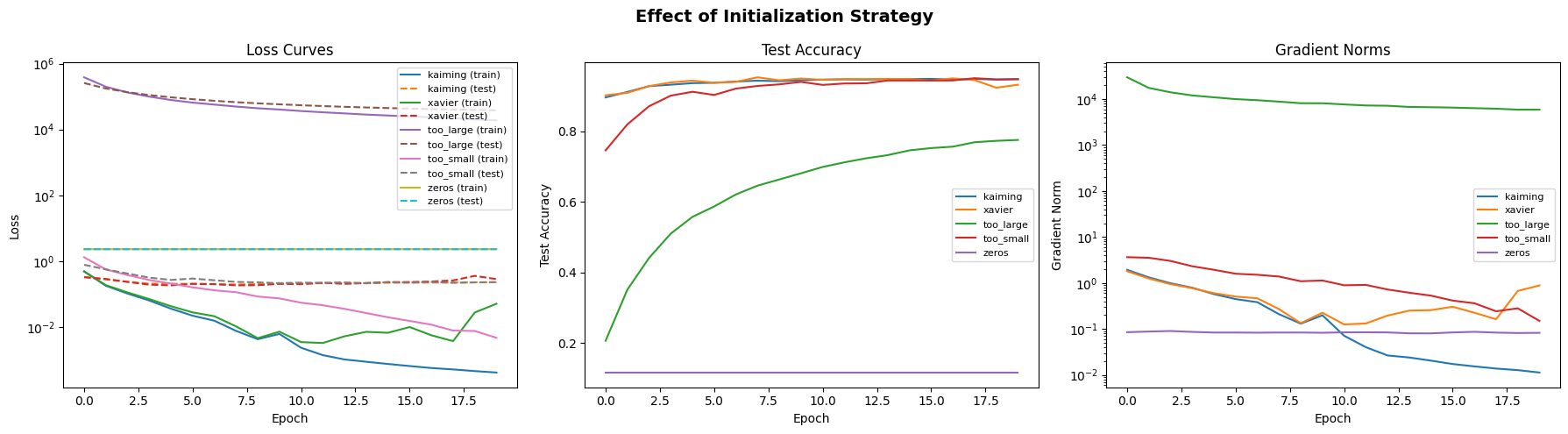
plot_histories(init_histories, "Effect of Initialization Strategy")

Training with different initializations...
(This may take a couple minutes)

--- kaiming ---

Epoch   1/20 | Train Loss: 0.4883 Acc: 0.847 | Test Loss: 0.3324 Acc: 0.896 | Grad Norm: 1.93 | LR: 1.00e-03

Epoch   6/20 | Train Loss: 0.0219 Acc: 0.995 | Test Loss: 0.2040 Acc: 0.938 | Grad Norm: 0.45 | LR: 1.00e-03

Epoch  11/20 | Train Loss: 0.0023 Acc: 1.000 | Test Loss: 0.2095 Acc: 0.947 | Grad Norm: 0.07 | LR: 1.00e-03

Epoch  16/20 | Train Loss: 0.0006 Acc: 1.000 | Test Loss: 0.2221 Acc: 0.949 | Grad Norm: 0.02 | LR: 1.00e-03

Epoch  20/20 | Train Loss: 0.0004 Acc: 1.000 | Test Loss: 0.2282 Acc: 0.949 | Grad Norm: 0.01 | LR: 1.00e-03

--- xavier ---

Epoch   1/20 | Train Loss: 0.4844 Acc: 0.850 | Test Loss: 0.3229 Acc: 0.902 | Grad Norm: 1.80 | LR: 1.00e-03

Epoch   6/20 | Train Loss: 0.0277 Acc: 0.993 | Test Loss: 0.2038 Acc: 0.938 | Grad Norm: 0.51 | LR: 1.00e-03

Epoch  11/20 | Train Loss: 0.0035 Acc: 1.000 | Test Loss: 0.1987 Acc: 0.947 | Grad Norm: 0.13 | LR: 1.00e-03

Epoch  16/20 | Train Loss: 0.0099 Acc: 0.998 | Test Loss: 0.2314 Acc: 0.944 | Grad Norm: 0.30 | LR: 1.00e-03

Epoch  20/20 | Train Loss: 0.0506 Acc: 0.982 | Test Loss: 0.2835 Acc: 0.932 | Grad Norm: 0.88 | LR: 1.00e-03

--- too_large ---

Epoch   1/20 | Train Loss: 382871.1685 Acc: 0.140 | Test Loss: 256255.1074 Acc: 0.207 | Grad Norm: 29741.88 | LR: 1.00e-03

Epoch   6/20 | Train Loss: 65256.3985 Acc: 0.654 | Test Loss: 82862.2471 Acc: 0.588 | Grad Norm: 9976.35 | LR: 1.00e-03

Epoch  11/20 | Train Loss: 36195.5532 Acc: 0.774 | Test Loss: 54214.9780 Acc: 0.700 | Grad Norm: 7647.51 | LR: 1.00e-03

Epoch  16/20 | Train Loss: 24765.9739 Acc: 0.829 | Test Loss: 43026.6458 Acc: 0.753 | Grad Norm: 6527.85 | LR: 1.00e-03

Epoch  20/20 | Train Loss: 18845.9009 Acc: 0.861 | Test Loss: 38035.2776 Acc: 0.776 | Grad Norm: 5886.94 | LR: 1.00e-03

--- too_small ---

Epoch   1/20 | Train Loss: 1.3082 Acc: 0.525 | Test Loss: 0.7722 Acc: 0.747 | Grad Norm: 3.64 | LR: 1.00e-03

Epoch   6/20 | Train Loss: 0.1597 Acc: 0.953 | Test Loss: 0.2950 Acc: 0.903 | Grad Norm: 1.59 | LR: 1.00e-03

Epoch  11/20 | Train Loss: 0.0543 Acc: 0.984 | Test Loss: 0.2215 Acc: 0.932 | Grad Norm: 0.89 | LR: 1.00e-03

Epoch  16/20 | Train Loss: 0.0152 Acc: 0.998 | Test Loss: 0.2220 Acc: 0.945 | Grad Norm: 0.41 | LR: 1.00e-03

Epoch  20/20 | Train Loss: 0.0047 Acc: 1.000 | Test Loss: 0.2292 Acc: 0.948 | Grad Norm: 0.15 | LR: 1.00e-03

--- zeros ---

Epoch   1/20 | Train Loss: 2.3022 Acc: 0.106 | Test Loss: 2.3018 Acc: 0.117 | Grad Norm: 0.08 | LR: 1.00e-03

Epoch   6/20 | Train Loss: 2.3007 Acc: 0.113 | Test Loss: 2.3011 Acc: 0.117 | Grad Norm: 0.08 | LR: 1.00e-03

Epoch  11/20 | Train Loss: 2.3002 Acc: 0.113 | Test Loss: 2.3011 Acc: 0.117 | Grad Norm: 0.08 | LR: 1.00e-03

Epoch  16/20 | Train Loss: 2.3006 Acc: 0.113 | Test Loss: 2.3010 Acc: 0.117 | Grad Norm: 0.08 | LR: 1.00e-03

Epoch  20/20 | Train Loss: 2.3006 Acc: 0.113 | Test Loss: 2.3012 Acc: 0.117 | Grad Norm: 0.08 | LR: 1.00e-03

Discussion

• Kaiming and Xavier both work well; Kaiming is theoretically better for ReLU.

• Too large (\(\sigma = 5\)): Activations explode, gradients are huge initially. May diverge or recover slowly.

• Too small (\(\sigma = 0.0001\)): Activations near zero, gradients tiny. Network barely learns.

• Zeros: Complete symmetry — all neurons compute the same function. No learning occurs.

Takeaway: Initialization is not a detail you can ignore. Use Kaiming for ReLU networks.

---

5. Experiment: Why Depth Is Hard (and How Normalization + Residuals Help)

Let’s try training deeper networks and see what breaks.

print("Training networks of different depths...\n")

depth_histories = {}

configs = [
    ('3 layers (baseline)',  dict(num_layers=3)),
    ('10 layers (plain)',    dict(num_layers=10)),
    ('10 layers + BN',      dict(num_layers=10, use_batchnorm=True)),
    ('10 layers + LN',      dict(num_layers=10, use_layernorm=True)),
    ('10 layers + Residual', dict(num_layers=10, use_residual=True)),
    ('10 layers + BN + Res', dict(num_layers=10, use_batchnorm=True, use_residual=True)),
]

for name, kwargs in configs:
    torch.manual_seed(42)
    model = make_mlp(hidden_dim=256, **kwargs)
    init_model(model, 'kaiming')

    print(f"--- {name} ({sum(p.numel() for p in model.parameters()):,} params) ---")
    h = train_model(model, train_loader, test_loader, epochs=25, lr=1e-3)
    depth_histories[name] = h
    print()

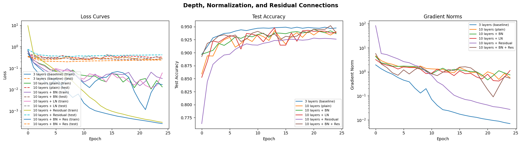
plot_histories(depth_histories, "Depth, Normalization, and Residual Connections")

Training networks of different depths...

--- 3 layers (baseline) (269,322 params) ---

Epoch   1/25 | Train Loss: 0.4883 Acc: 0.847 | Test Loss: 0.3324 Acc: 0.896 | Grad Norm: 1.93 | LR: 1.00e-03

Epoch   6/25 | Train Loss: 0.0219 Acc: 0.995 | Test Loss: 0.2040 Acc: 0.938 | Grad Norm: 0.45 | LR: 1.00e-03

Epoch  11/25 | Train Loss: 0.0023 Acc: 1.000 | Test Loss: 0.2095 Acc: 0.947 | Grad Norm: 0.07 | LR: 1.00e-03

Epoch  16/25 | Train Loss: 0.0006 Acc: 1.000 | Test Loss: 0.2221 Acc: 0.949 | Grad Norm: 0.02 | LR: 1.00e-03

Epoch  21/25 | Train Loss: 0.0004 Acc: 1.000 | Test Loss: 0.2308 Acc: 0.948 | Grad Norm: 0.01 | LR: 1.00e-03

Epoch  25/25 | Train Loss: 0.0003 Acc: 1.000 | Test Loss: 0.2339 Acc: 0.948 | Grad Norm: 0.01 | LR: 1.00e-03

--- 10 layers (plain) (729,866 params) ---

Epoch   1/25 | Train Loss: 0.5956 Acc: 0.817 | Test Loss: 0.4695 Acc: 0.859 | Grad Norm: 4.56 | LR: 1.00e-03

Epoch   6/25 | Train Loss: 0.0695 Acc: 0.977 | Test Loss: 0.2909 Acc: 0.929 | Grad Norm: 1.56 | LR: 1.00e-03

Epoch  11/25 | Train Loss: 0.0452 Acc: 0.987 | Test Loss: 0.2600 Acc: 0.935 | Grad Norm: 1.31 | LR: 1.00e-03

Epoch  16/25 | Train Loss: 0.0567 Acc: 0.986 | Test Loss: 0.3590 Acc: 0.916 | Grad Norm: 1.49 | LR: 1.00e-03

Epoch  21/25 | Train Loss: 0.0281 Acc: 0.992 | Test Loss: 0.3491 Acc: 0.934 | Grad Norm: 0.99 | LR: 1.00e-03

Epoch  25/25 | Train Loss: 0.0132 Acc: 0.996 | Test Loss: 0.3235 Acc: 0.941 | Grad Norm: 0.56 | LR: 1.00e-03

--- 10 layers + BN (734,474 params) ---

Epoch   1/25 | Train Loss: 0.6804 Acc: 0.784 | Test Loss: 0.3379 Acc: 0.897 | Grad Norm: 4.31 | LR: 1.00e-03

Epoch   6/25 | Train Loss: 0.0858 Acc: 0.972 | Test Loss: 0.3024 Acc: 0.921 | Grad Norm: 1.72 | LR: 1.00e-03

Epoch  11/25 | Train Loss: 0.0223 Acc: 0.994 | Test Loss: 0.2785 Acc: 0.935 | Grad Norm: 0.81 | LR: 1.00e-03

Epoch  16/25 | Train Loss: 0.0548 Acc: 0.987 | Test Loss: 0.2631 Acc: 0.936 | Grad Norm: 1.19 | LR: 1.00e-03

Epoch  21/25 | Train Loss: 0.0151 Acc: 0.996 | Test Loss: 0.2290 Acc: 0.945 | Grad Norm: 0.46 | LR: 1.00e-03

Epoch  25/25 | Train Loss: 0.0325 Acc: 0.992 | Test Loss: 0.2619 Acc: 0.936 | Grad Norm: 0.74 | LR: 1.00e-03

--- 10 layers + LN (734,474 params) ---

Epoch   1/25 | Train Loss: 0.5758 Acc: 0.828 | Test Loss: 0.4664 Acc: 0.853 | Grad Norm: 3.20 | LR: 1.00e-03

Epoch   6/25 | Train Loss: 0.0945 Acc: 0.970 | Test Loss: 0.2656 Acc: 0.933 | Grad Norm: 1.61 | LR: 1.00e-03

Epoch  11/25 | Train Loss: 0.0304 Acc: 0.991 | Test Loss: 0.3187 Acc: 0.932 | Grad Norm: 0.87 | LR: 1.00e-03

Epoch  16/25 | Train Loss: 0.0567 Acc: 0.985 | Test Loss: 0.3884 Acc: 0.914 | Grad Norm: 1.08 | LR: 1.00e-03

Epoch  21/25 | Train Loss: 0.0278 Acc: 0.992 | Test Loss: 0.3135 Acc: 0.941 | Grad Norm: 0.79 | LR: 1.00e-03

Epoch  25/25 | Train Loss: 0.0591 Acc: 0.984 | Test Loss: 0.2622 Acc: 0.939 | Grad Norm: 1.12 | LR: 1.00e-03

--- 10 layers + Residual (729,866 params) ---

Epoch   1/25 | Train Loss: 9.4918 Acc: 0.556 | Test Loss: 0.7590 Acc: 0.763 | Grad Norm: 82.10 | LR: 1.00e-03

Epoch   6/25 | Train Loss: 0.0749 Acc: 0.979 | Test Loss: 0.3660 Acc: 0.897 | Grad Norm: 2.63 | LR: 1.00e-03

Epoch  11/25 | Train Loss: 0.0079 Acc: 1.000 | Test Loss: 0.3629 Acc: 0.914 | Grad Norm: 0.71 | LR: 1.00e-03

Epoch  16/25 | Train Loss: 0.0010 Acc: 1.000 | Test Loss: 0.3848 Acc: 0.925 | Grad Norm: 0.08 | LR: 1.00e-03

Epoch  21/25 | Train Loss: 0.0005 Acc: 1.000 | Test Loss: 0.3992 Acc: 0.928 | Grad Norm: 0.04 | LR: 1.00e-03

Epoch  25/25 | Train Loss: 0.0003 Acc: 1.000 | Test Loss: 0.4142 Acc: 0.926 | Grad Norm: 0.03 | LR: 1.00e-03

--- 10 layers + BN + Res (734,474 params) ---

Epoch   1/25 | Train Loss: 0.7121 Acc: 0.848 | Test Loss: 0.3618 Acc: 0.892 | Grad Norm: 5.69 | LR: 1.00e-03

Epoch   6/25 | Train Loss: 0.0339 Acc: 0.989 | Test Loss: 0.2554 Acc: 0.931 | Grad Norm: 1.19 | LR: 1.00e-03

Epoch  11/25 | Train Loss: 0.0194 Acc: 0.994 | Test Loss: 0.2489 Acc: 0.941 | Grad Norm: 0.82 | LR: 1.00e-03

Epoch  16/25 | Train Loss: 0.0603 Acc: 0.984 | Test Loss: 0.2963 Acc: 0.931 | Grad Norm: 1.55 | LR: 1.00e-03

Epoch  21/25 | Train Loss: 0.0027 Acc: 0.999 | Test Loss: 0.2618 Acc: 0.945 | Grad Norm: 0.18 | LR: 1.00e-03

Epoch  25/25 | Train Loss: 0.0169 Acc: 0.995 | Test Loss: 0.2951 Acc: 0.939 | Grad Norm: 0.54 | LR: 1.00e-03

Discussion

• A plain 10-layer network often trains worse than a 3-layer one (the degradation problem).

• Batch/LayerNorm stabilize training by keeping activations well-scaled.

• Residual connections let gradients flow and make depth useful.

• BN + Residual together is typically the winning combination for deep MLPs.

This is exactly the insight behind ResNet, which made 100+ layer training practical.

---

6. Experiment: Learning Rate — The Most Important Hyperparameter

print("Training with different learning rates...\n")

lr_histories = {}

for lr in [1e-1, 1e-2, 1e-3, 1e-4, 1e-5]:
    torch.manual_seed(42)
    model = make_mlp(hidden_dim=256, num_layers=3)
    init_model(model, 'kaiming')

    print(f"--- LR = {lr} ---")
    h = train_model(model, train_loader, test_loader, epochs=20, lr=lr)
    lr_histories[f'lr={lr}'] = h
    print()

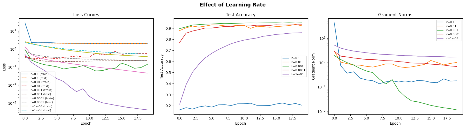
plot_histories(lr_histories, "Effect of Learning Rate")

Training with different learning rates...

--- LR = 0.1 ---

Epoch   1/20 | Train Loss: 27.7411 Acc: 0.181 | Test Loss: 2.1673 Acc: 0.163 | Grad Norm: 42.79 | LR: 1.00e-01

Epoch   6/20 | Train Loss: 2.1052 Acc: 0.180 | Test Loss: 2.0503 Acc: 0.188 | Grad Norm: 0.19 | LR: 1.00e-01

Epoch  11/20 | Train Loss: 1.9945 Acc: 0.210 | Test Loss: 2.0025 Acc: 0.218 | Grad Norm: 0.16 | LR: 1.00e-01

Epoch  16/20 | Train Loss: 1.9817 Acc: 0.206 | Test Loss: 1.9853 Acc: 0.215 | Grad Norm: 0.15 | LR: 1.00e-01

Epoch  20/20 | Train Loss: 1.9697 Acc: 0.216 | Test Loss: 1.9792 Acc: 0.204 | Grad Norm: 0.18 | LR: 1.00e-01

--- LR = 0.01 ---

Epoch   1/20 | Train Loss: 0.9060 Acc: 0.813 | Test Loss: 0.3794 Acc: 0.879 | Grad Norm: 2.94 | LR: 1.00e-02

Epoch   6/20 | Train Loss: 0.0998 Acc: 0.970 | Test Loss: 0.2812 Acc: 0.930 | Grad Norm: 0.69 | LR: 1.00e-02

Epoch  11/20 | Train Loss: 0.0854 Acc: 0.975 | Test Loss: 0.3542 Acc: 0.926 | Grad Norm: 0.67 | LR: 1.00e-02

Epoch  16/20 | Train Loss: 0.1607 Acc: 0.962 | Test Loss: 0.4870 Acc: 0.914 | Grad Norm: 1.21 | LR: 1.00e-02

Epoch  20/20 | Train Loss: 0.1365 Acc: 0.970 | Test Loss: 0.5549 Acc: 0.922 | Grad Norm: 1.00 | LR: 1.00e-02

--- LR = 0.001 ---

Epoch   1/20 | Train Loss: 0.4883 Acc: 0.847 | Test Loss: 0.3324 Acc: 0.896 | Grad Norm: 1.93 | LR: 1.00e-03

Epoch   6/20 | Train Loss: 0.0219 Acc: 0.995 | Test Loss: 0.2040 Acc: 0.938 | Grad Norm: 0.45 | LR: 1.00e-03

Epoch  11/20 | Train Loss: 0.0023 Acc: 1.000 | Test Loss: 0.2095 Acc: 0.947 | Grad Norm: 0.07 | LR: 1.00e-03

Epoch  16/20 | Train Loss: 0.0006 Acc: 1.000 | Test Loss: 0.2221 Acc: 0.949 | Grad Norm: 0.02 | LR: 1.00e-03

Epoch  20/20 | Train Loss: 0.0004 Acc: 1.000 | Test Loss: 0.2282 Acc: 0.949 | Grad Norm: 0.01 | LR: 1.00e-03

--- LR = 0.0001 ---

Epoch   1/20 | Train Loss: 1.2939 Acc: 0.600 | Test Loss: 0.7962 Acc: 0.772 | Grad Norm: 2.87 | LR: 1.00e-04

Epoch   6/20 | Train Loss: 0.1947 Acc: 0.946 | Test Loss: 0.3310 Acc: 0.902 | Grad Norm: 1.33 | LR: 1.00e-04

Epoch  11/20 | Train Loss: 0.1105 Acc: 0.972 | Test Loss: 0.2693 Acc: 0.920 | Grad Norm: 1.09 | LR: 1.00e-04

Epoch  16/20 | Train Loss: 0.0676 Acc: 0.987 | Test Loss: 0.2359 Acc: 0.931 | Grad Norm: 0.85 | LR: 1.00e-04

Epoch  20/20 | Train Loss: 0.0454 Acc: 0.993 | Test Loss: 0.2279 Acc: 0.931 | Grad Norm: 0.68 | LR: 1.00e-04

--- LR = 1e-05 ---

Epoch   1/20 | Train Loss: 2.5071 Acc: 0.148 | Test Loss: 2.2083 Acc: 0.213 | Grad Norm: 5.20 | LR: 1.00e-05

Epoch   6/20 | Train Loss: 1.0215 Acc: 0.725 | Test Loss: 1.1227 Acc: 0.673 | Grad Norm: 2.51 | LR: 1.00e-05

Epoch  11/20 | Train Loss: 0.6062 Acc: 0.841 | Test Loss: 0.7467 Acc: 0.792 | Grad Norm: 1.97 | LR: 1.00e-05

Epoch  16/20 | Train Loss: 0.4411 Acc: 0.883 | Test Loss: 0.5840 Acc: 0.845 | Grad Norm: 1.78 | LR: 1.00e-05

Epoch  20/20 | Train Loss: 0.3705 Acc: 0.902 | Test Loss: 0.5114 Acc: 0.860 | Grad Norm: 1.70 | LR: 1.00e-05

Discussion

• Too high (0.1): Loss may diverge or oscillate wildly.

• Just right (1e-3): Smooth convergence.

• Too low (1e-5): Training proceeds but painfully slowly.

In practice, you often sweep LR on a log scale (e.g., {1e-4, 3e-4, 1e-3, 3e-3, 1e-2}) as your first hyperparameter search.

---

7. Experiment: LR Schedules and Warmup

print("Comparing LR schedules...\n")

schedule_histories = {}

configs = [
    ('constant',         dict(lr=1e-3)),
    ('cosine decay',     dict(lr=1e-3, scheduler_type='cosine')),
    ('step decay',       dict(lr=1e-3, scheduler_type='step')),
    ('warmup + cosine',  dict(lr=1e-3, scheduler_type='cosine', warmup_epochs=3)),
    ('high LR + cosine', dict(lr=5e-3, scheduler_type='cosine', warmup_epochs=3)),
]

for name, kwargs in configs:
    torch.manual_seed(42)
    model = make_mlp(hidden_dim=256, num_layers=3)
    init_model(model, 'kaiming')

    print(f"--- {name} ---")
    h = train_model(model, train_loader, test_loader, epochs=30, **kwargs)
    schedule_histories[name] = h
    print()

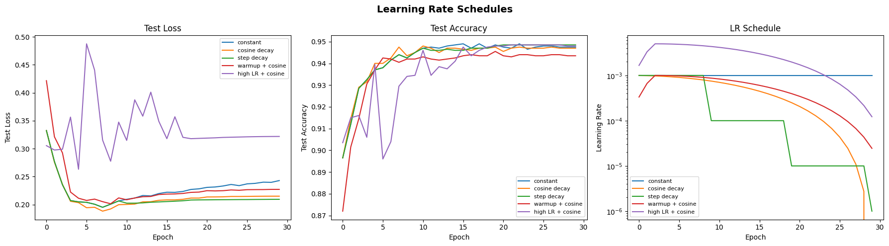
# Plot including LR schedule
fig, axes = plt.subplots(1, 3, figsize=(18, 5))

for name, h in schedule_histories.items():
    axes[0].plot(h['test_loss'], label=name)
axes[0].set_xlabel('Epoch')
axes[0].set_ylabel('Test Loss')
axes[0].set_title('Test Loss')
axes[0].legend(fontsize=8)

for name, h in schedule_histories.items():
    axes[1].plot(h['test_acc'], label=name)
axes[1].set_xlabel('Epoch')
axes[1].set_ylabel('Test Accuracy')
axes[1].set_title('Test Accuracy')
axes[1].legend(fontsize=8)

for name, h in schedule_histories.items():
    axes[2].plot(h['learning_rates'], label=name)
axes[2].set_xlabel('Epoch')
axes[2].set_ylabel('Learning Rate')
axes[2].set_title('LR Schedule')
axes[2].legend(fontsize=8)
axes[2].set_yscale('log')

plt.suptitle("Learning Rate Schedules", fontsize=14, fontweight='bold')
plt.tight_layout()
plt.show()

Comparing LR schedules...

--- constant ---

Epoch   1/30 | Train Loss: 0.4883 Acc: 0.847 | Test Loss: 0.3324 Acc: 0.896 | Grad Norm: 1.93 | LR: 1.00e-03

Epoch   6/30 | Train Loss: 0.0219 Acc: 0.995 | Test Loss: 0.2040 Acc: 0.938 | Grad Norm: 0.45 | LR: 1.00e-03

Epoch  11/30 | Train Loss: 0.0023 Acc: 1.000 | Test Loss: 0.2095 Acc: 0.947 | Grad Norm: 0.07 | LR: 1.00e-03

Epoch  16/30 | Train Loss: 0.0006 Acc: 1.000 | Test Loss: 0.2221 Acc: 0.949 | Grad Norm: 0.02 | LR: 1.00e-03

Epoch  21/30 | Train Loss: 0.0004 Acc: 1.000 | Test Loss: 0.2308 Acc: 0.948 | Grad Norm: 0.01 | LR: 1.00e-03

Epoch  26/30 | Train Loss: 0.0002 Acc: 1.000 | Test Loss: 0.2371 Acc: 0.948 | Grad Norm: 0.01 | LR: 1.00e-03

Epoch  30/30 | Train Loss: 0.0002 Acc: 1.000 | Test Loss: 0.2429 Acc: 0.948 | Grad Norm: 0.01 | LR: 1.00e-03

--- cosine decay ---

Epoch   1/30 | Train Loss: 0.4883 Acc: 0.847 | Test Loss: 0.3324 Acc: 0.896 | Grad Norm: 1.93 | LR: 9.97e-04

Epoch   6/30 | Train Loss: 0.0217 Acc: 0.996 | Test Loss: 0.1944 Acc: 0.940 | Grad Norm: 0.44 | LR: 9.05e-04

Epoch  11/30 | Train Loss: 0.0021 Acc: 1.000 | Test Loss: 0.2003 Acc: 0.948 | Grad Norm: 0.05 | LR: 7.03e-04

Epoch  16/30 | Train Loss: 0.0010 Acc: 1.000 | Test Loss: 0.2084 Acc: 0.947 | Grad Norm: 0.03 | LR: 4.48e-04

Epoch  21/30 | Train Loss: 0.0007 Acc: 1.000 | Test Loss: 0.2136 Acc: 0.946 | Grad Norm: 0.02 | LR: 2.06e-04

Epoch  26/30 | Train Loss: 0.0006 Acc: 1.000 | Test Loss: 0.2147 Acc: 0.947 | Grad Norm: 0.02 | LR: 4.32e-05

Epoch  30/30 | Train Loss: 0.0006 Acc: 1.000 | Test Loss: 0.2150 Acc: 0.947 | Grad Norm: 0.02 | LR: 0.00e+00

--- step decay ---

Epoch   1/30 | Train Loss: 0.4883 Acc: 0.847 | Test Loss: 0.3324 Acc: 0.896 | Grad Norm: 1.93 | LR: 1.00e-03

Epoch   6/30 | Train Loss: 0.0219 Acc: 0.995 | Test Loss: 0.2040 Acc: 0.938 | Grad Norm: 0.45 | LR: 1.00e-03

Epoch  11/30 | Train Loss: 0.0024 Acc: 1.000 | Test Loss: 0.2025 Acc: 0.947 | Grad Norm: 0.07 | LR: 1.00e-04

Epoch  16/30 | Train Loss: 0.0015 Acc: 1.000 | Test Loss: 0.2054 Acc: 0.946 | Grad Norm: 0.03 | LR: 1.00e-04

Epoch  21/30 | Train Loss: 0.0012 Acc: 1.000 | Test Loss: 0.2085 Acc: 0.949 | Grad Norm: 0.03 | LR: 1.00e-05

Epoch  26/30 | Train Loss: 0.0012 Acc: 1.000 | Test Loss: 0.2090 Acc: 0.949 | Grad Norm: 0.03 | LR: 1.00e-05

Epoch  30/30 | Train Loss: 0.0012 Acc: 1.000 | Test Loss: 0.2094 Acc: 0.949 | Grad Norm: 0.03 | LR: 1.00e-06

--- warmup + cosine ---

Epoch   1/30 | Train Loss: 0.7120 Acc: 0.783 | Test Loss: 0.4217 Acc: 0.872 | Grad Norm: 2.14 | LR: 3.33e-04

Epoch   6/30 | Train Loss: 0.0346 Acc: 0.991 | Test Loss: 0.2074 Acc: 0.943 | Grad Norm: 0.61 | LR: 9.76e-04

Epoch  11/30 | Train Loss: 0.0025 Acc: 1.000 | Test Loss: 0.2086 Acc: 0.943 | Grad Norm: 0.07 | LR: 8.35e-04

Epoch  16/30 | Train Loss: 0.0011 Acc: 1.000 | Test Loss: 0.2188 Acc: 0.944 | Grad Norm: 0.03 | LR: 6.04e-04

Epoch  21/30 | Train Loss: 0.0007 Acc: 1.000 | Test Loss: 0.2249 Acc: 0.944 | Grad Norm: 0.02 | LR: 3.45e-04

Epoch  26/30 | Train Loss: 0.0006 Acc: 1.000 | Test Loss: 0.2267 Acc: 0.944 | Grad Norm: 0.02 | LR: 1.28e-04

Epoch  30/30 | Train Loss: 0.0005 Acc: 1.000 | Test Loss: 0.2272 Acc: 0.944 | Grad Norm: 0.01 | LR: 2.45e-05

--- high LR + cosine ---

Epoch   1/30 | Train Loss: 0.4559 Acc: 0.860 | Test Loss: 0.3055 Acc: 0.903 | Grad Norm: 1.86 | LR: 1.67e-03

Epoch   6/30 | Train Loss: 0.0679 Acc: 0.978 | Test Loss: 0.4876 Acc: 0.896 | Grad Norm: 0.71 | LR: 4.88e-03

Epoch  11/30 | Train Loss: 0.0360 Acc: 0.987 | Test Loss: 0.3148 Acc: 0.946 | Grad Norm: 0.55 | LR: 4.17e-03

Epoch  16/30 | Train Loss: 0.0048 Acc: 0.999 | Test Loss: 0.3179 Acc: 0.948 | Grad Norm: 0.13 | LR: 3.02e-03

Epoch  21/30 | Train Loss: 0.0001 Acc: 1.000 | Test Loss: 0.3189 Acc: 0.948 | Grad Norm: 0.00 | LR: 1.73e-03

Epoch  26/30 | Train Loss: 0.0001 Acc: 1.000 | Test Loss: 0.3212 Acc: 0.949 | Grad Norm: 0.00 | LR: 6.42e-04

Epoch  30/30 | Train Loss: 0.0000 Acc: 1.000 | Test Loss: 0.3219 Acc: 0.948 | Grad Norm: 0.00 | LR: 1.22e-04

---

8. Experiment: Batch Size and the LR—Batch Size Relationship

print("Batch size experiments...\n")
print("The linear scaling rule says: when you multiply batch size by k, multiply LR by k.\n")
print("NOTE: We use SGD here — adaptive optimizers (Adam) mask the effect.\n")

bs_histories = {}

base_lr = 1e-2
base_bs = 64

configs = [
    (f'bs={base_bs}, lr={base_lr}', base_bs, base_lr),
    (f'bs={base_bs*4}, lr={base_lr} (WRONG)', base_bs * 4, base_lr),
    (f'bs={base_bs*4}, lr={base_lr*4} (scaled)', base_bs * 4, base_lr * 4),
    (f'bs=16, lr={base_lr/4} (scaled down)', 16, base_lr / 4),
]

for name, bs, lr in configs:
    torch.manual_seed(42)
    model = make_mlp(hidden_dim=256, num_layers=3)
    init_model(model, 'kaiming')

    loader = DataLoader(train_subset, batch_size=bs, shuffle=True)

    print(f"--- {name} ---")
    h = train_model(model, loader, test_loader, epochs=20, lr=lr, optimizer_type='sgd')
    bs_histories[name] = h
    print()

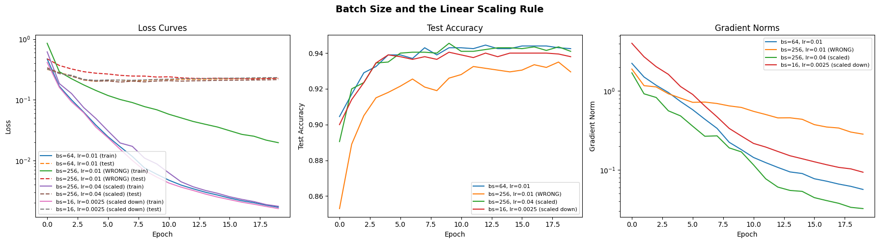
plot_histories(bs_histories, "Batch Size and the Linear Scaling Rule")

Batch size experiments...

The linear scaling rule says: when you multiply batch size by k, multiply LR by k.

NOTE: We use SGD here — adaptive optimizers (Adam) mask the effect.

--- bs=64, lr=0.01 ---

Epoch   1/20 | Train Loss: 0.4688 Acc: 0.854 | Test Loss: 0.3172 Acc: 0.904 | Grad Norm: 2.24 | LR: 1.00e-02

Epoch   6/20 | Train Loss: 0.0246 Acc: 0.996 | Test Loss: 0.2086 Acc: 0.939 | Grad Norm: 0.58 | LR: 1.00e-02

Epoch  11/20 | Train Loss: 0.0047 Acc: 1.000 | Test Loss: 0.2149 Acc: 0.943 | Grad Norm: 0.14 | LR: 1.00e-02

Epoch  16/20 | Train Loss: 0.0024 Acc: 1.000 | Test Loss: 0.2218 Acc: 0.944 | Grad Norm: 0.08 | LR: 1.00e-02

Epoch  20/20 | Train Loss: 0.0017 Acc: 1.000 | Test Loss: 0.2277 Acc: 0.943 | Grad Norm: 0.06 | LR: 1.00e-02

--- bs=256, lr=0.01 (WRONG) ---

Epoch   1/20 | Train Loss: 0.8517 Acc: 0.726 | Test Loss: 0.4728 Acc: 0.853 | Grad Norm: 1.90 | LR: 1.00e-02

Epoch   6/20 | Train Loss: 0.1175 Acc: 0.969 | Test Loss: 0.2656 Acc: 0.921 | Grad Norm: 0.72 | LR: 1.00e-02

Epoch  11/20 | Train Loss: 0.0578 Acc: 0.987 | Test Loss: 0.2392 Acc: 0.928 | Grad Norm: 0.55 | LR: 1.00e-02

Epoch  16/20 | Train Loss: 0.0309 Acc: 0.996 | Test Loss: 0.2241 Acc: 0.930 | Grad Norm: 0.37 | LR: 1.00e-02

Epoch  20/20 | Train Loss: 0.0196 Acc: 0.999 | Test Loss: 0.2254 Acc: 0.929 | Grad Norm: 0.28 | LR: 1.00e-02

--- bs=256, lr=0.04 (scaled) ---

Epoch   1/20 | Train Loss: 0.6156 Acc: 0.807 | Test Loss: 0.3362 Acc: 0.890 | Grad Norm: 1.70 | LR: 4.00e-02

Epoch   6/20 | Train Loss: 0.0307 Acc: 0.994 | Test Loss: 0.2043 Acc: 0.940 | Grad Norm: 0.36 | LR: 4.00e-02

Epoch  11/20 | Train Loss: 0.0062 Acc: 1.000 | Test Loss: 0.2063 Acc: 0.941 | Grad Norm: 0.12 | LR: 4.00e-02

Epoch  16/20 | Train Loss: 0.0025 Acc: 1.000 | Test Loss: 0.2097 Acc: 0.943 | Grad Norm: 0.04 | LR: 4.00e-02

Epoch  20/20 | Train Loss: 0.0018 Acc: 1.000 | Test Loss: 0.2148 Acc: 0.941 | Grad Norm: 0.03 | LR: 4.00e-02

--- bs=16, lr=0.0025 (scaled down) ---

Epoch   1/20 | Train Loss: 0.4122 Acc: 0.874 | Test Loss: 0.3213 Acc: 0.900 | Grad Norm: 4.03 | LR: 2.50e-03

Epoch   6/20 | Train Loss: 0.0236 Acc: 0.996 | Test Loss: 0.2122 Acc: 0.938 | Grad Norm: 0.91 | LR: 2.50e-03

Epoch  11/20 | Train Loss: 0.0043 Acc: 1.000 | Test Loss: 0.2180 Acc: 0.939 | Grad Norm: 0.22 | LR: 2.50e-03

Epoch  16/20 | Train Loss: 0.0023 Acc: 1.000 | Test Loss: 0.2272 Acc: 0.940 | Grad Norm: 0.13 | LR: 2.50e-03

Epoch  20/20 | Train Loss: 0.0016 Acc: 1.000 | Test Loss: 0.2321 Acc: 0.938 | Grad Norm: 0.09 | LR: 2.50e-03

Discussion

• Increasing batch size without scaling LR → effectively lower LR per data point → slower training.

• The linear scaling rule corrects for this: multiply LR proportionally with batch size.

• Very large batch sizes eventually break the linear scaling rule and need more careful treatment (e.g., LARS/LAMB optimizers, extended warmup).

---

9. Experiment: Gradient Clipping in Action

print("Demonstrating gradient clipping...")
print("We'll use a deliberately unstable setup (high LR, deep network, no normalization)\n")

clip_histories = {}

for clip_val, label in [(None, 'no clipping'), (1.0, 'clip=1.0'), (0.1, 'clip=0.1')]:
    torch.manual_seed(42)
    # Deliberately challenging: deep, no norm, somewhat high LR
    model = make_mlp(hidden_dim=256, num_layers=6)
    init_model(model, 'kaiming')

    print(f"--- {label} ---")
    h = train_model(
        model, train_loader, test_loader,
        epochs=20, lr=5e-3, grad_clip=clip_val
    )
    clip_histories[label] = h
    print()

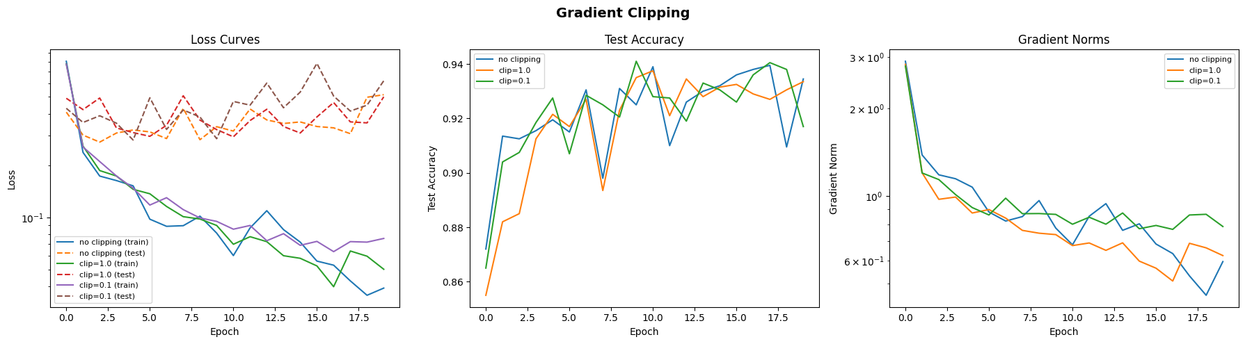
plot_histories(clip_histories, "Gradient Clipping")

Demonstrating gradient clipping...
We'll use a deliberately unstable setup (high LR, deep network, no normalization)

--- no clipping ---

Epoch   1/20 | Train Loss: 0.8049 Acc: 0.774 | Test Loss: 0.4081 Acc: 0.872 | Grad Norm: 2.90 | LR: 5.00e-03

Epoch   6/20 | Train Loss: 0.0978 Acc: 0.971 | Test Loss: 0.3136 Acc: 0.915 | Grad Norm: 0.88 | LR: 5.00e-03

Epoch  11/20 | Train Loss: 0.0602 Acc: 0.982 | Test Loss: 0.3170 Acc: 0.939 | Grad Norm: 0.68 | LR: 5.00e-03

Epoch  16/20 | Train Loss: 0.0559 Acc: 0.984 | Test Loss: 0.3369 Acc: 0.936 | Grad Norm: 0.68 | LR: 5.00e-03

Epoch  20/20 | Train Loss: 0.0390 Acc: 0.989 | Test Loss: 0.5152 Acc: 0.934 | Grad Norm: 0.59 | LR: 5.00e-03

--- clip=1.0 ---

Epoch   1/20 | Train Loss: 0.7771 Acc: 0.794 | Test Loss: 0.4910 Acc: 0.855 | Grad Norm: 2.83 | LR: 5.00e-03

Epoch   6/20 | Train Loss: 0.1373 Acc: 0.964 | Test Loss: 0.2955 Acc: 0.917 | Grad Norm: 0.90 | LR: 5.00e-03

Epoch  11/20 | Train Loss: 0.0700 Acc: 0.981 | Test Loss: 0.2936 Acc: 0.938 | Grad Norm: 0.68 | LR: 5.00e-03

Epoch  16/20 | Train Loss: 0.0524 Acc: 0.986 | Test Loss: 0.3828 Acc: 0.932 | Grad Norm: 0.56 | LR: 5.00e-03

Epoch  20/20 | Train Loss: 0.0501 Acc: 0.989 | Test Loss: 0.5008 Acc: 0.933 | Grad Norm: 0.62 | LR: 5.00e-03

--- clip=0.1 ---

Epoch   1/20 | Train Loss: 0.7748 Acc: 0.789 | Test Loss: 0.4296 Acc: 0.865 | Grad Norm: 2.79 | LR: 5.00e-03

Epoch   6/20 | Train Loss: 0.1181 Acc: 0.968 | Test Loss: 0.4945 Acc: 0.907 | Grad Norm: 0.86 | LR: 5.00e-03

Epoch  11/20 | Train Loss: 0.0855 Acc: 0.981 | Test Loss: 0.4708 Acc: 0.928 | Grad Norm: 0.80 | LR: 5.00e-03

Epoch  16/20 | Train Loss: 0.0727 Acc: 0.985 | Test Loss: 0.7825 Acc: 0.926 | Grad Norm: 0.79 | LR: 5.00e-03

Epoch  20/20 | Train Loss: 0.0756 Acc: 0.987 | Test Loss: 0.6202 Acc: 0.917 | Grad Norm: 0.79 | LR: 5.00e-03

Discussion

• Without clipping, a deep network with high LR can see gradient spikes that blow up training.

• Gradient clipping acts as a safety net: it doesn’t change the gradient direction, just bounds its magnitude.

• Typical clip value: 1.0. If you need very aggressive clipping (0.01), something else is probably wrong.

---

10. Experiment: Gradient Accumulation

print("Gradient accumulation: simulating a larger batch size\n")
print("Effective batch size = micro_batch_size × accumulation_steps\n")

accum_histories = {}

# Baseline: batch size 256 with scaled LR
torch.manual_seed(42)
model = make_mlp(hidden_dim=256, num_layers=3)
init_model(model, 'kaiming')
loader_256 = DataLoader(train_subset, batch_size=256, shuffle=True)
print("--- bs=256 (actual) ---")
h = train_model(model, loader_256, test_loader, epochs=20, lr=4e-2, optimizer_type='sgd')
accum_histories['bs=256 (actual)'] = h
print()

# Simulated: batch size 64 × 4 accumulation steps = effective 256
torch.manual_seed(42)
model = make_mlp(hidden_dim=256, num_layers=3)
init_model(model, 'kaiming')
loader_64 = DataLoader(train_subset, batch_size=64, shuffle=True)
print("--- bs=64 × 4 accum = 256 (simulated) ---")
h = train_model(model, loader_64, test_loader, epochs=20, lr=4e-2, optimizer_type='sgd', accumulation_steps=4)
accum_histories['bs=64×4 (accumulated)'] = h
print()

# For comparison: actual batch size 64
torch.manual_seed(42)
model = make_mlp(hidden_dim=256, num_layers=3)
init_model(model, 'kaiming')
print("--- bs=64 (no accumulation) ---")
h = train_model(model, loader_64, test_loader, epochs=20, lr=1e-2, optimizer_type='sgd')
accum_histories['bs=64 (no accum)'] = h
print()

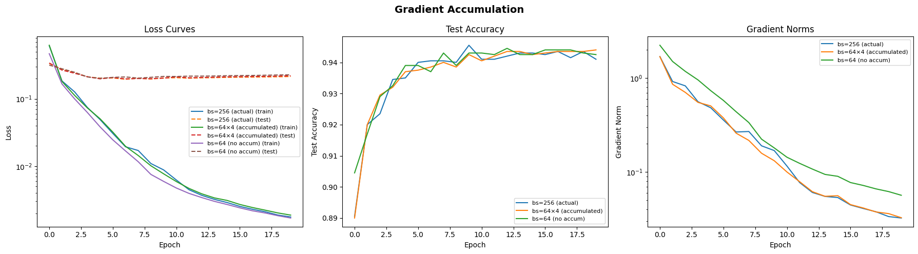
plot_histories(accum_histories, "Gradient Accumulation")

Gradient accumulation: simulating a larger batch size

Effective batch size = micro_batch_size × accumulation_steps

--- bs=256 (actual) ---

Epoch   1/20 | Train Loss: 0.6156 Acc: 0.807 | Test Loss: 0.3362 Acc: 0.890 | Grad Norm: 1.70 | LR: 4.00e-02

Epoch   6/20 | Train Loss: 0.0307 Acc: 0.994 | Test Loss: 0.2043 Acc: 0.940 | Grad Norm: 0.36 | LR: 4.00e-02

Epoch  11/20 | Train Loss: 0.0062 Acc: 1.000 | Test Loss: 0.2063 Acc: 0.941 | Grad Norm: 0.12 | LR: 4.00e-02

Epoch  16/20 | Train Loss: 0.0025 Acc: 1.000 | Test Loss: 0.2097 Acc: 0.943 | Grad Norm: 0.04 | LR: 4.00e-02

Epoch  20/20 | Train Loss: 0.0018 Acc: 1.000 | Test Loss: 0.2148 Acc: 0.941 | Grad Norm: 0.03 | LR: 4.00e-02

--- bs=64 × 4 accum = 256 (simulated) ---

Epoch   1/20 | Train Loss: 0.6259 Acc: 0.807 | Test Loss: 0.3409 Acc: 0.890 | Grad Norm: 1.70 | LR: 4.00e-02

Epoch   6/20 | Train Loss: 0.0321 Acc: 0.993 | Test Loss: 0.2072 Acc: 0.938 | Grad Norm: 0.38 | LR: 4.00e-02

Epoch  11/20 | Train Loss: 0.0059 Acc: 1.000 | Test Loss: 0.2116 Acc: 0.941 | Grad Norm: 0.10 | LR: 4.00e-02

Epoch  16/20 | Train Loss: 0.0027 Acc: 1.000 | Test Loss: 0.2138 Acc: 0.943 | Grad Norm: 0.04 | LR: 4.00e-02

Epoch  20/20 | Train Loss: 0.0019 Acc: 1.000 | Test Loss: 0.2199 Acc: 0.944 | Grad Norm: 0.03 | LR: 4.00e-02

--- bs=64 (no accumulation) ---

Epoch   1/20 | Train Loss: 0.4688 Acc: 0.854 | Test Loss: 0.3172 Acc: 0.904 | Grad Norm: 2.24 | LR: 1.00e-02

Epoch   6/20 | Train Loss: 0.0246 Acc: 0.996 | Test Loss: 0.2086 Acc: 0.939 | Grad Norm: 0.58 | LR: 1.00e-02

Epoch  11/20 | Train Loss: 0.0047 Acc: 1.000 | Test Loss: 0.2149 Acc: 0.943 | Grad Norm: 0.14 | LR: 1.00e-02

Epoch  16/20 | Train Loss: 0.0024 Acc: 1.000 | Test Loss: 0.2218 Acc: 0.944 | Grad Norm: 0.08 | LR: 1.00e-02

Epoch  20/20 | Train Loss: 0.0017 Acc: 1.000 | Test Loss: 0.2277 Acc: 0.943 | Grad Norm: 0.06 | LR: 1.00e-02

Discussion

Gradient accumulation lets you simulate large batch sizes when your GPU can’t fit them. The accumulated version should closely match the actual large-batch training (up to differences in batch normalization statistics, if used).

This is essential when:

• You’re fine-tuning large models on limited hardware

• Your data samples are large (e.g., high-res images, long sequences)

• You want to scale up without changing hardware

---

11. Monitoring with Weights & Biases

Everything above was tracked locally. In real projects, you’ll want a centralized dashboard. Weights & Biases (wandb) is the most popular option.

# Uncomment and run this cell to try wandb integration
# You'll need a free wandb account: https://wandb.ai/authorize

USE_WANDB = False  # Set to True to enable

if USE_WANDB:
    import wandb

    # Log in (will prompt for API key in Colab)
    wandb.login()

    # Start a run
    wandb.init(
        project="binf4002-nn-lab",
        name="demo-run",
        config={
            "architecture": "MLP",
            "hidden_dim": 256,
            "num_layers": 3,
            "learning_rate": 1e-3,
            "batch_size": 128,
            "optimizer": "adam",
            "dataset": "MNIST",
        }
    )

    torch.manual_seed(42)
    model = make_mlp(hidden_dim=256, num_layers=3)
    init_model(model, 'kaiming')

    h = train_model(
        model, train_loader, test_loader,
        epochs=20, lr=1e-3, use_wandb=True,
        run_name='demo-run'
    )

    # Log final model
    wandb.finish()
    print("\n✅ Check your wandb dashboard for interactive plots!")
else:
    print("Set USE_WANDB = True above to try Weights & Biases integration.")
    print("\nWhat you would see in the wandb dashboard:")
    print("  • Interactive loss/accuracy curves")
    print("  • Gradient norm tracking")
    print("  • LR schedule visualization")
    print("  • System metrics (GPU util, memory)")
    print("  • Side-by-side comparison of runs")
    print("  • Hyperparameter search visualization")

Set USE_WANDB = True above to try Weights & Biases integration.

What you would see in the wandb dashboard:
  • Interactive loss/accuracy curves
  • Gradient norm tracking
  • LR schedule visualization
  • System metrics (GPU util, memory)
  • Side-by-side comparison of runs
  • Hyperparameter search visualization

---

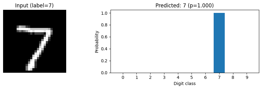
12. Visualizing What the Network Learns

Let’s peek inside our trained network.

# Use the baseline model we trained earlier
baseline_model.eval()

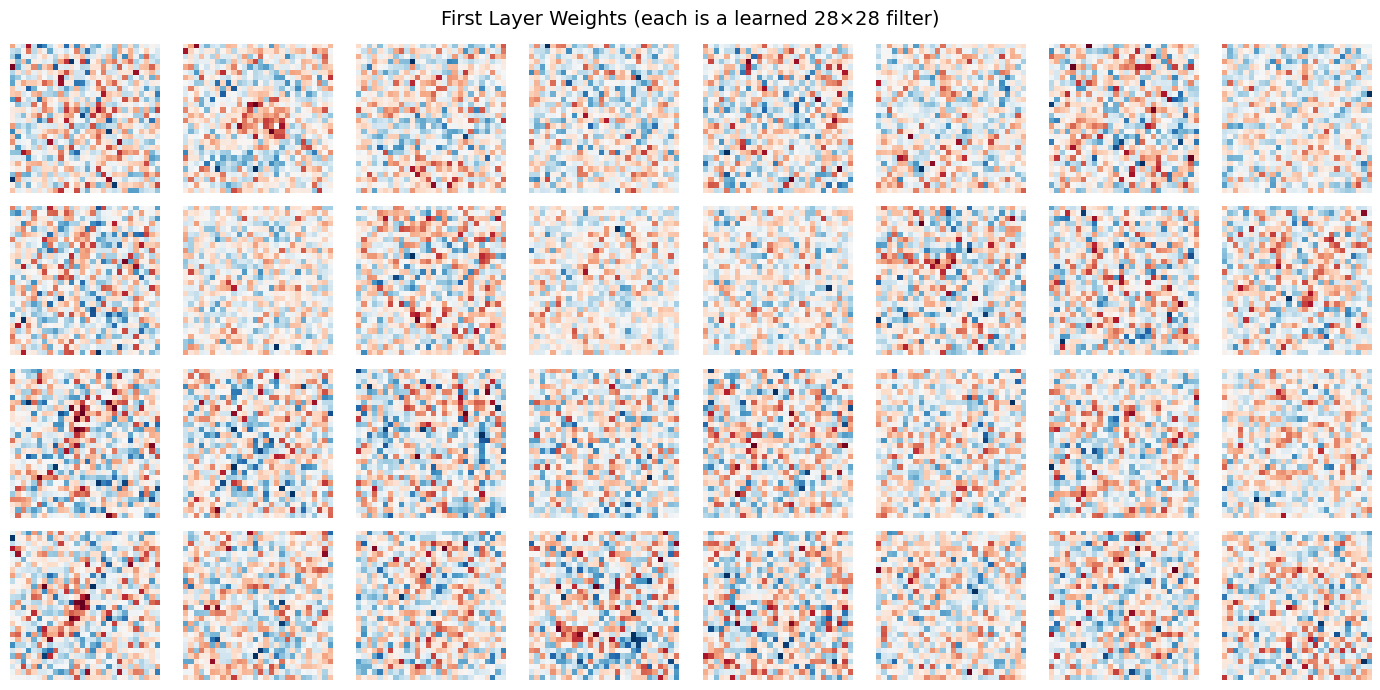
# Visualize first-layer weights as 28×28 images
# Each row of W1 is a 784-dim vector that can be reshaped to 28×28
first_layer = list(baseline_model.blocks[0].parameters())[0] # First weight matrix
weights = first_layer.detach().cpu().numpy()

fig, axes = plt.subplots(4, 8, figsize=(14, 7))
for i, ax in enumerate(axes.flat):
    if i < weights.shape[0]:
        w = weights[i].reshape(28, 28)
        ax.imshow(w, cmap='RdBu', vmin=-w.max(), vmax=w.max())
    ax.axis('off')
plt.suptitle("First Layer Weights (each is a learned 28×28 filter)", fontsize=14)
plt.tight_layout()
plt.show()

# Visualize activations for a single input
baseline_model.eval()
sample_img, sample_label = test_dataset[0]
x = sample_img.unsqueeze(0).to(device)

# Forward pass, capturing intermediates
activations = []
h = x.view(1, -1)
for block in baseline_model.blocks:
    h = block(h)
    activations.append(h.detach().cpu().numpy().flatten())

fig, axes = plt.subplots(1, len(activations), figsize=(16, 3))
for i, (act, ax) in enumerate(zip(activations, axes)):
    ax.bar(range(len(act[:50])), act[:50], width=1.0)  # Show first 50 dims
    ax.set_title(f"Layer {i+1} (first 50 dims)")
    ax.set_xlabel("Neuron")
    if i == 0:
        ax.set_ylabel("Activation")

plt.suptitle(f"Activations for a '{sample_label}' digit (showing first 50 neurons per layer)", fontsize=13)
plt.tight_layout()
plt.show()

# Show the prediction
with torch.no_grad():
    logits = baseline_model(sample_img.unsqueeze(0).to(device))
    probs = torch.softmax(logits, dim=1).cpu().numpy().flatten()

fig, (ax1, ax2) = plt.subplots(1, 2, figsize=(10, 3))
ax1.imshow(sample_img.squeeze(), cmap='gray')
ax1.set_title(f"Input (label={sample_label})")
ax1.axis('off')

ax2.bar(range(10), probs)
ax2.set_xlabel('Digit class')
ax2.set_ylabel('Probability')
ax2.set_title(f'Predicted: {probs.argmax()} (p={probs.max():.3f})')
ax2.set_xticks(range(10))
plt.tight_layout()
plt.show()

---

13. Summary: What We’ve Learned

Concept	Key Takeaway
Layers	act(Wx + b) — the fundamental building block
Initialization	Use Kaiming for ReLU; bad init → no learning
Normalization	BatchNorm/LayerNorm stabilize deep training
Residual connections	Essential for training deep networks
Learning rate	Most important hyperparameter; sweep on log scale
LR schedules	Warmup + cosine decay is a strong default
Batch size ↔ LR	Linear scaling rule: scale LR with batch size
Gradient clipping	Safety net for unstable training
Gradient accumulation	Simulate large batches on small GPUs
Monitoring	Track loss, accuracy, grad norms, LR with wandb

Next Steps

Try modifying these experiments:

• Change the activation function (GELU, tanh, sigmoid) — what changes?

• Add dropout and compare generalization (train-test gap)

• Try SGD with momentum instead of Adam

• Increase to the full MNIST dataset (60K training samples)

• Replace the MLP with a simple CNN and compare

print("🎉 Lab complete! See the lecture slides for the conceptual framework behind everything here.")

🎉 Lab complete! See the lecture slides for the conceptual framework behind everything here.